Hidden Markov Models

April 21, 2025 · 8 min read · Page View:

Random Process | Hidden Markov Models | Math

If you have any questions, feel free to comment below.

This is a lecture note of Hidden Markov Models.

HIDDEN MARKOV MODEL (HMM) #

Want to recognize patterns (e.g.sequence motifs), we have to learn from the data. Applications include gene prediction and stock price and trading.

Markov chain can predict the future given the present, dependent only on the previous (or current) state with transition probabilities.

Many problems can’t be solved by a Markov model due to unknown or hard-to-assess states. For example, in speech recognition.
A hidden Markov model (HMM) is a Markov model where probabilities are based in part on hidden states. HMMs need to be trained, for example, in gene finding with nucleotide sequences or stock price prediction with known patterns.

WEATHER FORECASTING #

On any day, the weather can be rainy/snowy, cloudy or sunny. Given a probability matrix for weather transitions.

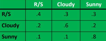
To compute a sequence, we multiply them together, so if today is sunny then the probability that the next two days will be sunny is $0.8\times0.8$, and the probability that the next two days will be cloudy is $0.1\times0.6\times0.6$.

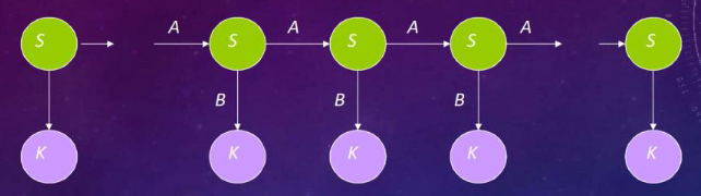
WHAT IS AN HMM? #

Graphical Model

Green circles are hidden states, dependent only on the previous state.
Purple nodes are observed states, dependent only on their corresponding hidden state.
Arrows indicate probabilistic dependencies between states.

HMM FORMALISM #

An HMM is represented by ${S,K,\Pi,A,B}$:
- $S={s_{1}… s_{N}}$ are the values for the hidden states.
- $K={k_{1}… k_{M}}$ are the values for the observations.
- $\Pi={\pi_{1}}$ are the initial state probabilities.
- $A={a_{ij}}$ are the state transition probabilities.
- $B={b_{ik}}$ are the observation state probabilities (output probabilities).

INFERENCE IN AN HMM #

Problem 1: Evaluation - Compute the probability of a given observation sequence.
Problem 2: Decoding - Given an observation sequence, compute the most likely hidden state sequence.
Problem 3: Learning - Given an observation sequence and set of possible models, which model most closely fits the data?

EXAMPLE:SPEECH RECOGNITION #

We have acoustic signal observations, but the intention (phonemes/words) that created the signal is hidden.
The goal is to identify the actual utterance by adding hidden states and appropriate probabilities for transitions.
The observables are not states in our network, but transition links.

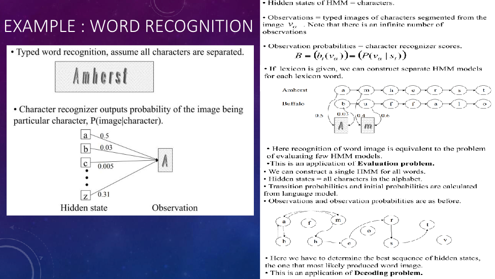
EXAMPLE:WORD RECOGNITION #

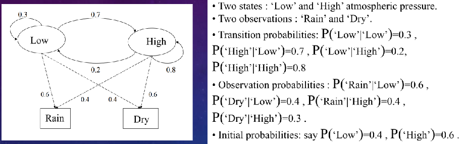
EXAMPLE HMM: WEATHER FORECASTING #

TRELLIS REPRESENTATION OF AN HMM #

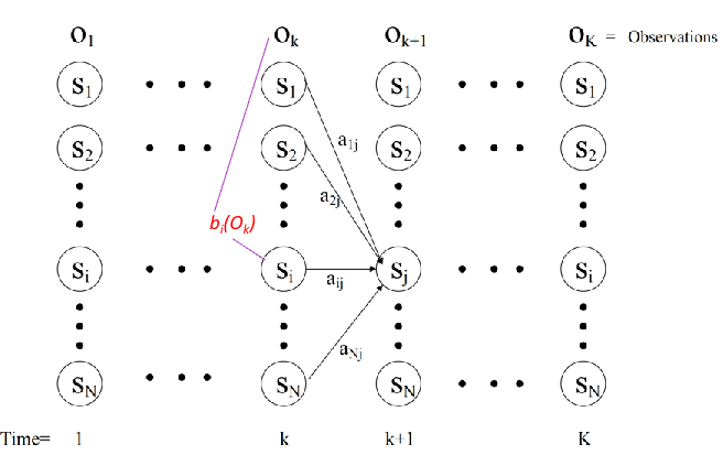
HMM PROBLEM 1 Evaluation #

Given an HMM(hidden markov model sequence) and an output sequence(observation sequence), compute the probability of generating that particular output sequence.

$$ p_{s1} * b_{s1}(O_1) * a_{s1s2} * b_{s2}(O_2) * a_{s2s3} * b_{s3}(O_3) * ... * a_{s_{n - 1}s_n} * b_{s_n}(O_n) $$

p is the initial state probability.
$a$ is the state transition probability.
$b$ is the output probability.

Example #

We have:

3 time units,t1,t2,t3
each has 2 states, s1,s2
- p(s1 at t1)=.8
- p(s2 at t1)=.2
- Pi = [0.8 0.2]
3 possible outputs A, B, C

Our transition probabilities a are:

p(s1,s1)=.7
p(s1,s2)=.3
p(s2,s2)=.6
p(s2,s1)=.4
${A} = \begin{bmatrix} 0.7 & 0.3 \ 0.4 & 0.6 \end{bmatrix}$

Our output probabilities b are:

p(A|s1)=.5
p(B|s1)=.4
p(C|s1)=.1
p(A|s2)=.7
p(B|s2)=.3
p(C|s2)=.0
${B} = \begin{bmatrix} 0.5 & 0.4 & 0.1 \ 0.7 & 0.3 & 0 \end{bmatrix}$

What is the probability of generating A, B, C?

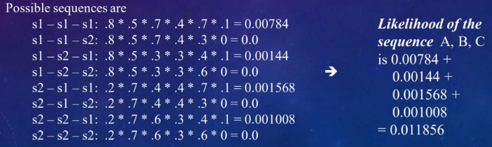
We want to compute the probability of the output sequence A,B,C

THE FORWARD ALGORITHM #

Initialization step: $\alpha_{1}(i)=\pi_{i}^{*}b_{i}(O_{1})$ for all states $i$, which is the probabilities of starting at each initial state i at t1.
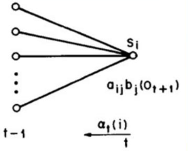
Main step (recursive): $\alpha_{t + 1}(j)=[\sum\alpha_{t}(i)*a_{ij}]*b_{j}(O_{t+1})$ for all states $j$ at time $t+1$.
- $\alpha_{t}(i)$ is the previous probability of being in state $i$ at time $t$.
- $a_{ij}$ is the probability of transitioning from state $i$ to state $j$.
- $b_{j}(O_{t+1})$ is the probability of observing the output $O_{t+1}$ given that we are in state $j$.
Final step: Sum up the probabilities of ending in each of the states at time $n$. $\sum_{i}\alpha_{n}(i)$

HMM PROBLEM 2 Decoding #

Given a sequence of observations, compute the optimal sequence of state transitions that would cause those observations. Alternatively, we could say that the optimal sequence best explains the observations.

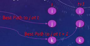
THE VITERBI ALGORITHM #

Use recursion and dynamic programming.
Initialization step:
- $\alpha_{i}(i)=\pi_{i}^{*}b_{i}(O_{1})$
- $\psi_{1}(0)=0$ this array will represent the state that maximized our path leading to the prior state.
Recursive step:
- $\delta_{t + 1}(j)=\max[\alpha_{i}(i)*a_{ij}]*b_{j}(O_{t+1})$, here we are maximizing the probability of the path leading to the current state.
- $\psi_{t + 1}(j)=\arg\max[\alpha_{i}(i)*a_{ij}]$, here we are storing the state that maximizes the probability of the path leading to the current state.
Termination step:
- $p^*=\max_{i}[\delta_{n}(i)]$，$n$ this the last step. Find the largest probability in the final time step.
- When the optimal path probability $p^$ and the terminating state $q^$ are determined, the path backtracking is used to get the best path. Starting from $\psi[q^*]$, step by step backtracking until the first time step.

VITERBI IN PSEUDOCODE #

def forvard_viterb(obs,states,start_p,transp,emit_p):
    T = {}
    for state in states:
        T[state]=(start_p[state],[state],start_p[state])
    for output in obs:
        U = {}
        for next_state in states:
            total = 0
            argmax = None
            valmax = 0
            for source_state in states:
                p = emit_p[source_state][output]
                prob_t = p * T[source_state][2] * transp[source_state][next_state]
                total += prob_t
                if T[source_state][2]*transp[source_state][next_state]>valmax:
                    argmax = T[source_state][1]+[next_state]
                    valmax = T[source_state][2]*transp[source_state][next_state]
            U[next_state]=(total,argmax,valmax)
        T = U
    total = 0
    valmax = 0
    argmax = None
    for state in states:
        prob = T[state][0]
        total += prob
        if T[state][2]>valmax:
            argmax = T[state][1]
            valmax = T[state][2]
    return (total,argmax,valmax)

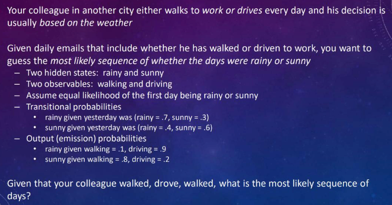
HOMEWORK! Sunny or Rainy? #

WHY PROBLEM 2? #

Applications, The HMM and Viterbi give us the ability to generate the best explanation where the term best means the most likely sequence through all of the states:
- given a speech signal, what was uttered what phonemes or words were uttered)?
- given a set of symptoms, what disease(s) is the patient suffering from?
- given a misspelled word, which word was intended?
- given a series of events, what caused them?
HOW DO WE OBTAIN OUR PROBABILITIES?
- Need prior probabilities, transition probabilities, and output (emission) probabilities.
- Can accumulate probabilities through counting, but it may be difficult to get accurate probabilities, especially output probabilities.
- This leads to HMM problem 3.

HMM PROBLEM 3 Learning #

Given HMM and output sequence, update the various probabilities. Solved by the Baum-Welch algorithm (also known as the Estimation-Modification or EM algorithm), which uses the forward-backward algorithm.

FORWARD-BACKWARD #

Compute forward probabilities as in the Forward algorithm.
Backward portion:
- Initialization step: $\beta_{t}(i)=1$, also start from time t, but as initial point.
- $\beta_{t}(i)=1= P(O_{t+1}, O_{t+2}… O_{K} | \text{state is i at t})$, Joint probability of the partial observation sequence $O_{t+1}, O_{t+2}… O_{K}$ given that the hidden state at time k is state i. The Backward probability.
- Recursive step: $$ \beta_{t}(i)=\sum a_{ij}*b_{j}(O_{t + 1})*\beta_{t+1}(j) $$
- $b_{j}(O_{t + 1})$ is the probability of state j given out $O_{t + 1}$.

BAUM-WELCH (EM) #

Compute

$$ \xi_{t}(i,j)=\frac{\alpha_{t}(i)*a_{ij}*b_{j}(O_{t+1})*\beta_{t+1}(j)}{\text{denominator}} $$

where the denominator normalizes the probabilities.

forward $\alpha_{t}(i)$
backward $\beta_{t+1}(j)$
trans $a_{ij}$
output $O_{t+1}$
Compute $\gamma_{t}(i)=\sum\xi_{t}(i,j)$ for all $j$ at time $t$.
- This represents the expected number of times we are at state i at time t
- If we sum up $\gamma_{t}(i)$ for all times t, we have the number of expected times we are i state i.
Re-estimation: Update probabilities based on the expected number of times in a state or transition. Start with estimated probabilities, use training examples to adjust, and continue until probabilities stabilize.
Our observation probabilities $b_{i}(O_{t})$: p(observation i | state j )=(expected number of times we saw observation i in the test case / number of times we achieved state j )
Our transition probabilities $a_{ij}$: p(state i | state j) (expected number of transitions from i to j / number of times we were in state j )
this is the prior probability: $\pi(\text{state } i)=\alpha_{1}(i) * \beta_{1}(i)/\sum_{i}[\alpha_{1}(i) * \beta_{1}(i)] \text{ for all states } i$

Some advantages:

Start with estimated probabilities (they don’t even have to be very good)
- The better the initial probabilities, the more likely it will be that the algorithm will converge to a stable state quickly, the worse the initial probabilities, the longer it will take.
Use training examples to adjust the probabilities
And continue until the probabilities stabilize: that is, between iterations of Baum-Welch, they do not change (or their change is less than a given error rate)
- So HMMs can be said to learn the proper probabilities through training examples

HMM CAVEATS #

States may not be independent.
If a probability (output or transition) is 0, it can cause issues that the path will never be selected. Replace 0 probabilities with a minimum value (e.g., 0.001).
Need to be mindful of overfitting and require a good training set. More training data doesn’t always mean a better model.
Recall that the complexity for the forward algorithm is $O(T*N^T)$ where N is 30(hidden states 30 phonemes) and T is 100(utterance around 100 phonemes-20 words)!
High complexity in search, especially for long sequences. Can use beam search to reduce the number of possible paths searched.

BEAM SEARCH #

A combination of heuristic and breadth-first search. Examine all next states, evaluate them (using $\alpha$ or $\beta$ in HMMs), and retain only some states (either top $k$ or above a threshold value).

APPLICATIONS FOR HMMS #

Speech recognition (1980s)
Hand - written character recognition
Natural language understanding
- Word sense disambiguation
- Machine translation
- Word matching (for misspelled words)
- Semantic tagging of words
Bioinformatics (protein structure predictions, gene analysis and sequencing predictions)
Market predictions
Diagnosis of mechanical systems

PREDICT STOCK - MARKET BEHAVIOR WITH MARKOV CHAINS AND PYTHON #

Markov Chain offers a probabilistic approach to predict the likelihood of an event based on prior behavior.
Analyze market behavior, create transition matrices, bin values, combine event features, and create two Markov Chains (for volume jumps and drops) to predict future stock-market outcomes.