Markov Chains
April 20, 2025 · 27 min read · Page View:
If you have any questions, feel free to comment below. And if you think it's helpful to you, just click on the ads which can support this site. Thanks!
This is the notes for the lecture of Markov Chains.
- OUTLINE
- Markov Chain
- Transition Probability
- Examples and applications
- CHAPMAN-KOLMOGOROV EQUATION
- Classification of States
- Stationary Distribution and Limiting Prob
- Ergodicity
- Markov Chain
MARKOV CHAIN #
A special kind of Markov process, where the system can occupy a finite or countably infinite number of states $e_0,e_1,e_2,\cdots$ such that the future evolution of the process, once it is in a given state, depends only on the present state and not on how it arrived at that state. It can be discrete or continuous.
MARKOV PROPERTY #
A sequence of random variables $(X_t)$ is called a Markov chain if it has the Markov property: $P(X_t = x_t|X_{t - 1}=x_{t - 1},X_{t - 2}=x_{t - 2},\cdots,X_0=x_0)=P(X_t = x_t|X_{t - 1}=x_{t - 1})$
- States are usually labelled ${x_0,x_1,x_2,\cdots}$ and state space can be finite or infinite.
- First order Markov assumption (memoryless).
- Homogeneity: $P(X_{m + n}=x_j|X_m=x_i)=P(X_n=x_j|X_0=x_i)$
Example #
1-D RANDOM WALK #
Time is slotted.
The walker flips a coin every time slot to decide which way to go: $X(t + 1)=\begin{cases}X(t)+1& \text{with probability }p\X(t)-1& \text{with probability }(1 - p)\end{cases}$
- The sequence of Bernoulli trials $Y_1,Y_2,\cdots$ at each stage are independent, and the accumulated partial sum $S_n=X_1 + X_2+\cdots+X_n$, $S_{n + 1}=S_n+X_{n + 1}$
- $P(S_{n + 1}=j + 1|S_n=j)=p$
- $P(S_{n + 1}=j - 1|S_n=j)=q$
- Conditional probabilities for $S_n$ depend only on the values of $S_n$ and are not affected by the values of $S_1,S_2,\cdots,S_{n - 1}$
BRANCHING PROCESSES #
Time is discrete and represents successive generations.
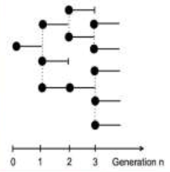
- Each individual has a unit lifetime, at the end of which it might give birth to one or more offsprings simultaneously.
- The offspring distribution is described by a random variable $\xi$ taking non-negative integer values with corresponding probabilities $p_k = P[\xi=k], k\geq0$
- All individuals behave independently of each other.
- The population size at generation $n$ is denoted by $Z_n$, where $\xi_{i,n}$ are iid. copies of $\xi$, representing the number of offspring of the $i$ - th member of the $(n - 1)$ generation.
- The process ${Z_n,n\geq0}$ is a discrete-time Markov chain on the state space ${0,1,2,3,\cdots}$ where state $0$ is absorbing and all other states are transient.
NUCLEAR CHAIN REACTION #
- A particle such as a neutron scores a hit with probability $p$, creating $m$ new particles, and $q = 1 - p$ represents the probability that it remains inactive with no descendants.
- The only possible number of descendants is zero and $m$ with probabilities $q$ and $p$.
- If $p$ is close to one, the number of particles is likely to increase indefinitely, leading to an explosion, whereas if $p$ is close to zero the process may never start.
WAITING LINES/QUEUES #
- Customers (jobs) arrive randomly and wait for service.
- A customer arriving when the server is free receives immediate service; otherwise the customer joins the queue and waits for service.
- The server continues service according to some schedule such as first in, first out.
- Busy period: total duration of uninterrupted service at some $t = t_0$
TRANSITION PROBABILITIES #
In a discrete-time Markov chain ${X_n}$ with a finite or infinite set of states $e_1,e_2,\cdots,e_N$
- Let $X_n = X(t_n)$ represent the state of the system at $t=t_n$.
- For $n\geq m\geq0$, the sequence $X_m,X_{m + 1},\cdots,X_n$ represents the evolution of the system.
- Let $p_i(m)=P(X_m = e_i)$ be the probability that at time $t = t_m$ the system is in state $e_i$.
- $p_{ij}(m,n)=P(X_n = e_j|X_m = e_i)$ be the probability that the system goes into state $e_j$ at $t=t_n$ given that it was in state $e_i$ at $t=t_m$ (transition probabilities of the Markov chain from state $e_i$ at $t_m$ to $e_j$ at $t_n$).
- For $m\lt n\lt r$, $P{X_r = e_i,X_n = e_j,X_m = e_k}=P{X_r = e_i|X_n = e_j}P{X_n = e_j|X_m = e_k}P{X_m = e_k}=p_{ji}(n,r)p_{kj}(m,n)p_k(m)$
HOMOGENEOUS MARKOV CHAIN #
- Homogeneous: if $p_{ij}(m,n)$ depends only on the difference $n-m$.
- The transition probabilities are stationary and $P{X_{m + n}=e_j|X_m = e_i}\triangleq p_{ij}(n)=p_{ij}^{(n)}$
- One-step transition probabilities: $p_{ij}=P(X_{n+1}=e_j|X_n = e_i)$ is the basic transition.
- The time duration $Y$ that a homogeneous Markov process spends in a given state (interarrival time) must be memoryless. $P(y>m + n|y>m)=P(y>n)$, y is a geometric random variable.
STOCHASTIC MATRIX #
- Arrange the transition probabilities $p_{ij}(m,n)$ in a matrix form $P(m,n)$ $$ P(m,n)=\begin{pmatrix}p_{11}(m,n)&p_{12}(m,n)&\cdots&p_{1N}(m,n)&\cdots\\p_{21}(m,n)&p_{22}(m,n)&\cdots&\cdots&\cdots\\\vdots&\vdots&\vdots&\vdots&\vdots\\p_{N1}(m,n)&\cdots&\cdots&p_{NN}(m,n)&\cdots\\\cdots&\cdots&\cdots&\cdots&\cdots\end{pmatrix} $$
where $\sum_{j}p_{ij}(m,n)=\sum_{j}P[X_n = e_j|X_m = e_i]=1$ (elements of each row sums to 1).
With the initial distribution $p(m)=P(X_m = e_i)$ for some $m$, $P(m,n)$ completely define the Markov chain.
For a homogeneous MC,(refer to the definition of homogeneous Markov chain)
$$ P=\begin{pmatrix}p_{11}&p_{12}&p_{13}&\cdots&p_{1N}&\cdots\\p_{21}&p_{22}&p_{23}&\cdots&\cdots&\cdots\\p_{31}&p_{32}&p_{23}&\cdots&\cdots&\cdots\\\vdots&\vdots&\vdots&\vdots&\vdots&\vdots\\p_{N1}&p_{N2}&p_{N3}&\cdots&p_{NN}&\cdots\\\cdots&\cdots&\cdots&\cdots&\cdots&\cdots\end{pmatrix} $$EXAMPLE - BINARY COMMUNICATION CHANNEL #
The channel delivers the input symbol to the output with a certain error probability that may depend on the symbol being transmitted.
Let $\alpha\lt\frac{1}{2}$ and $\beta\lt\frac{1}{2}$ represent the two kinds of channel error probabilities.
- For a time-invariant channel, these error probabilities remain constant over various transmitted Symbols so that $P{X_{n + 1}=1|X_n = 0}=p_{01}=\alpha$, $P{X_{n + 1}=0|X_n = 1}=p_{10}=\beta$
- The corresponding Markov chain is homogeneous.
- $2\times2$ homogeneous probability transition matrix $$ P=\begin{pmatrix}P_{00}&P_{01}\\p_{10}&p_{11}\end{pmatrix}=\begin{pmatrix}1-\alpha&\alpha\\\beta&1 - \beta\end{pmatrix} $$
EXAMPLE - Weather Forecasting #
Suppose that the chance of rain tomorrow depends on previous weather conditions only through whether or not it is raining today and not on past weather conditions.
Suppose also that if it rains today, then it will rain tomorrow with probability $\alpha$; and if it does not rain today, then it will rain tomorrow with probability $\beta$.
- Let’s denote that the process is in state $0$ (the first state) when it rains and state $1$ (the second state) when it does not.
- $P=\begin{pmatrix}\alpha&1-\alpha\\beta&1 - \beta\end{pmatrix}$
EXAMPLE – Mood of Gary #
On any given day Gary is either cheerful (C), so-so (S), or glum (G).
- If he is cheerful today, then he will be C, S, or G tomorrow with respective probabilities $0.5$, $0.4$, $0.1$.
- If he feels so-so today, then he will be C, S, or G tomorrow with probabilities $0.3$, $0.4$, $0.3$.
- If he is glum today, then he will be C, S, or G tomorrow with probabilities $0.2$, $0.3$, $0.5$.
Let $X_n$ denote Gary’s mood on the $n$-th day, then ${X_n,n\geq0}$ is a three - state Markov chain (state $0 = C$, state $1 = S$, state $2 = G$) with transition probability matrix
$$ P=\begin{pmatrix}0.5&0.4&0.1\\0.3&0.4&0.3\\0.2&0.3&0.5\end{pmatrix} $$EXAMPLE - Transforming a (non-Markov) Process into a Markov Chain #
Suppose that whether or not it rains today depends on previous weather conditions through the last two days.
Specifically, suppose that if it has rained for the past two days, then it will rain tomorrow with probability $0.7$; if it rained today but not yesterday, then it will rain tomorrow with probability $0.5$; if it rained yesterday but not today, then it will rain tomorrow with probability $0.4$; if it has not rained in the past two days, then it will rain tomorrow with probability $0.2$.
If we let the state at time $n$ depend only on whether or not it is raining at time $n - 1$, then the preceding model is not a Markov chain. But we can transform this model into a Markov chain by saying that the state at any time is determined by the weather conditions during both that day and the previous day.
- state $0$ if it rained both today and yesterday
- state $1$ if it rained today but not yesterday
- state $2$ if it rained yesterday but not today
- state $3$ if it did not rain either yesterday or today.
The transition probability matrix
$$ P=\begin{pmatrix}0.7&0&0.3&0\\0.5&0&0.5&0\\0&0.4&0&0.6\\0&0.2&0&0.8\end{pmatrix} $$eg. $p_{02}=0.3$ means the probability changes from state 0 to state 2 is 0.3.
EXAMPLE - BACK TO RANDOM WALK #
At each interior state $e_i$ the particle move to:
- the right to $e_{i + 1}$ with probability $p$
- to the left to $e_{i - 1}$ with probability $q$
- remains at $e_i$ with probability $r$.
Let $n$ represent the location of the particle at time $n$ on a straight line.
$$ P=\begin{pmatrix}r_0&p_0&0&0&0&\cdots\\q_1&r_1&p_1&0&0&\cdots\\0&q_2&r_2&p_2&0&\cdots\\0&0&q_3&r_3&p_3&\cdots\\\vdots&\vdots&\vdots&\vdots&\vdots&\vdots\end{pmatrix} $$- With $p_i = p$, $q_i = 1 - p$, $r_i = 0$ for $i>1$, and $r_0 = 1$ → the gambler’s ruin problem
RANDOM WALK WITH ABSORBING BARRIERS in the edge nodes #
Special case: if the number of states in a random walk be finite $(e_0,e_1,\cdots,e_N)$
From the interior states $e_1,e_2,\cdots,e_{N - 1}$ transitions to the left and right neighbors are with probabilities $q$ and $p$ respectively, while no transition is possible from $e_0$ and $e_N$ to any other state.
$$ P=\begin{pmatrix}1&0&0&0&\cdots&0\\q&0&p&0&0&\vdots\\0&q&0&p&0&\cdots\\\vdots&\vdots&\vdots&\vdots&\vdots&\vdots\\0&0&\cdots&\cdots&q&0&p\\0&0&\cdots&\cdots&0&0&1\end{pmatrix} $$RANDOM WALK WITH REFLECTING BARRIERS #
If the two boundaries in the previous example reflect the particle back to the adjacent state instead of absorbing it, with $e_1,e_2,\cdots,e_N$ representing the $N$ states.
The end reflection probabilities to the right and left are given by $p_{10}=p$ and $p_{N,N - 1}=q$
$$ P=\begin{pmatrix}q&p&0&0&\cdots&0\\q&0&p&0&0&\cdots\\0&q&0&p&0&\cdots\\\vdots&\vdots&\vdots&\vdots&\vdots&\vdots\\0&0&0&\cdots&0&p\\0&0&0&\cdots&0&q&p\end{pmatrix} $$A fun game where every time a player loses the game, his adversary returns just the stake amount so that the game is kept alive and it continues forever
CYCLIC RANDOM WALKS #
The two end-boundary states $e_1$ and $e_N$ loop together to form a circle so that $e_N$ has neighbors $e_1$ and $e_{N - 1}$.
$$ P=\begin{pmatrix}0&p&0&0&\cdots&0&q\\q&0&p&0&\cdots&0&0\\0&q&0&p&\cdots&0&0\\\vdots&\vdots&\vdots&\vdots&\vdots&\vdots&\vdots\\0&0&0&\cdots&0&p&0\\p&0&0&\cdots&0&q&0\end{pmatrix} $$If we permit transition between any two states $e_i$ and $e_j$, then since moving $k$ steps to the right on a circle is the same as moving $N - k$ to the left, the transition probability matrix is symmetric.
$$ P=\begin{pmatrix}q_0&q_1&q_2&\cdots&q_{N - 1}\\q_{N - 1}&q_0&q_1&\cdots&q_{N - 2}\\q_{N - 2}&q_{N - 1}&q_0&\cdots&q_{N - 3}\\\vdots&\vdots&\vdots&\vdots&\vdots\\q_1&q_2&\cdots&q_{N - 1}&q_0\end{pmatrix} $$$$ q_{k}=P\left\{x_{n+1}=e_{i + k} | x_{k}=e_{i}\right\}=P\left\{x_{n+1}=e_{i-(N - k)} | x_{n}=e_{i}\right\} $$EHRENFEST’S DIFFUSION MODEL (NON-UNIFORM RANDOM WALK) #
Let $N$ represent the combined population of two cities $A$ and $B$. Suppose migration occurs between the cities one at a time with probability proportional to the population of the city, and let the population of $A$ determine the state of the system. Then $e_0,e_1,\cdots,e_N$ represent the possible states, and from state $e_k$ at the next step, $A$ can move into either $e_{k + 1}$ or $e_{k - 1}$ with probabilities $k/N$ or $1 - k/N$ respectively
$$ P=\begin{pmatrix}0&1&0&0&\cdots&0&0\\p&0&1-p&0&\cdots&0&0\\0&2p&0&1-2p&\cdots&0&0\\0&0&3p&0&1-3p&\cdots&0\\\vdots&\vdots&\vdots&\vdots&\vdots&\vdots&\vdots\\0&0&0&\cdots&0&1-p&0\\0&0&0&\cdots&0&1-p&0\\0&0&0&\cdots&0&0&1\end{pmatrix} $$A random walk with totally reflective barriers where the probability of a step varies with the position of state. If $k\leq N/2$, the particle is more likely to move to the right, while if $k > N/2$, it is more likely to move to the left.
The particle has a tendency to move toward the center, an equilibrium distribution.
SUCCESS RUNS (RANDOM WALK) #
$p$ - success, $q$ - failure
The particle moves from $i$ to $i + 1$ with probability $p$ or moves back to the origin with probability $q$.
$$ p_{ij}= \begin{cases}p & j = i + 1 \\ q & j = 0 \\ 0 & otherwise \end{cases} $$$$ \prod p_i=p $$$e_i$ represents the number of uninterrupted successes up to the $n$th trial
$$ More generally p_{ij}= \begin{cases}p_i & j = i + 1 \\ q_i & j = 0 \\ 0 & otherwise \end{cases} $$The probability that the time between two successive returns to zero equals $k$ is given by the product $p_1p_2\cdots p_{k - 1}q$.
RANDOM OCCUPANCY #
A sequence of independent trials is conducted where a new ball is placed at random into one of the $N$ cells at each trial. Each cell can hold multiple balls.
Let $e_k$, $k = 0,1,\cdots,N$ represent the state where $k$ cells are occupied and $N - k$ cells are empty.
At the next trial, the next ball can go into one of the occupied cells ($e_k$ to $e_k$) with probability $k/N$ or an empty cell ($e_k$ to $e_{k+1}$) with probability $(N - k)/N$.
The transition probabilities:
$$ p_{kk}=\frac{k}{N} \quad \text{and} \quad p_{k,k + 1}=1-\frac{k}{N}, \quad p_{kj}=0\ (j\neq k,j\neq k + 1) $$Birthday statistics problem: What is the minimum number of people required in a random group so that every day is a birthday for someone in that group (with probability $p$)?
IMBEDDED MARKOV CHAINS #
An imbedded Markov chain $(X_n)$ that represents the number of customers or jobs waiting for service in a queue at the departure of the $n$th customer.
Let $X_n$ be the number of customers waiting for service at the departure of the $n$-th customer.
The number of customers waiting for service at the departure of the $(n + 1)$st customer is
$$ x_{n+1}= \begin{cases}x_{n}+y_{n+1}-1 & x_{n} \neq 0\\y_{n+1} & x_{n}=0\end{cases} $$Let $Y_n$ denote the number of customers arriving at the queue during the service time of the $n$th customer.
If the queue was empty at the departure of the $n$th customer, then $X_n = 0$, and the next customer to arrive is the $(n + 1)$st. During that service, $Y_{n+1}$ customers arrive, so that $X_{n+1}=Y_{n+1}$; otherwise the number of customers left behind by the $(n + 1)$st customer is $X_n-1+Y_{n+1}$. The transition probabilities
$$ \alpha_{j}=P\left(x_{n+1}=j | x_{n}=i\right)= \begin{cases}P\left(y_{n+1}=j\right) & i = 0\\P\left(y_{n+1}=j - i + 1\right) & i\geq1\end{cases} $$Note that the underlying stochastic process $X_t$ need not be Markovian, whereas the sequence $X_n = X(t_n)$ generated at the random departure time instants $t_n$ is Markovian.
The method of imbedded Markov chains converts a non-Markovian problem into Markovian, and the limiting behavior of the imbedded chain can be used to study the underlying process.
$$ P=\begin{pmatrix}a_0&a_1&a_2&a_3&\ddots&\ddots\\a_0&a_1&a_2&a_3&\ddots&\ddots\\0&a_0&a_1&a_2&\ddots&\ddots\\0&0&a_0&a_1&\ddots&\ddots\\\vdots&\vdots&\vdots&\vdots&\vdots&\vdots\end{pmatrix} $$$$ \lim _{t \to \infty} P(x(t)=k)=\lim _{n \to \infty} P\left(x_{n}=k\right) $$for certain queues after a long time, i.e., the limiting behavior at a stationary state is the same as those at the random departure instant.
CHAPMAN KOLMOGOROV EQUATION #
Remember?
$$ \begin{aligned} P\left(x_{r}=e_{i}, x_{n}=e_{j}, x_{m}=e_{k}\right) &=P\left(x_{r}=e_{i} | x_{m}=e_{j}\right)P\left(x_{n}=e_{j} | x_{m}=e_{k}\right)P\left(x_{m}=e_{k}\right) \\ &=p_{ji}(n,r)p_{kj}(m,n)p_{k}(m) \end{aligned} $$For $n>m$
$$ \begin{aligned} P\left(x_{n}=e_{j}, x_{m}=e_{i}\right) &=\sum_{k} P\left(x_{n}=e_{j}, x_{k}=e_{k}, x_{m}=e_{i}\right) \\ &=\sum_{k} P\left(x_{n}=e_{j} | x_{k}=e_{k}, x_{m}=e_{i}\right)P\left(x_{k}=e_{k}, x_{m}=e_{i}\right) \\ &=\sum_{k} P\left(x_{n}=e_{j} | x_{k}=e_{k}\right)P\left(x_{k}=e_{k} | x_{m}=e_{i}\right) \end{aligned} $$$$ \begin{aligned} p_{ij}(m,n) &=P\left(x_{n}=e_{j} | x_{m}=e_{i}\right) \\ &=\sum_{k} P\left(x_{n}=e_{j} | x_{k}=e_{k}\right)P\left(x_{k}=e_{k} | x_{m}=e_{i}\right) \end{aligned} $$$$ p_{ij}(m,n)=\sum_{k} p_{ik}(m,r)p_{kj}(r,n) $$By letting $r=m + 1,m + 2,\cdots$
$$ P(m,n)=P(m,m + 1)P(m + 1,m + 2)\cdots P(n - 1,n) $$For all $n>m$, it is sufficient to know the one-step transition probability matrices $P(0,1),P(1,2),\cdots,P(n - 1,n)$.
For a homogeneous Markov chain, $P(i,i + 1)=P$, for all $i$ → $P(m,n)=P^{n - m}$.
N-STEP TRANSITION PROBABILITIES #
For a homogeneous chain $p_{ij}^{(n)}$ represents the $(i,j)$th entry of $P(0,n)=P^n$. As $p_{ij}^{(m + n)}=p_{ik}^{(m)}p_{kj}^{(n)}=p_{ik}^{(n)}p_{kj}^{(m)}$, we have:
$$ p_{ij}^{(m + n)}=\sum_{k} p_{ik}^{(m)}p_{kj}^{(n)}=\sum_{k} p_{ik}^{(n)}p_{kj}^{(m)} $$The one-step recursion relation
$$ p_{ij}^{(n+1)}=\sum_{k} p_{ik}p_{kj}^{(n)}=\sum_{k} p_{ik}^{(n)}p_{kj} $$The unconditional probability distribution at $t=nT$, or $p(n)=p(m)p(m,n)$, where
$$ p(n) \triangleq\left[p_1(n),p_2(n),\cdots,p_j(n),\cdots\right] $$$$ \begin{aligned} p_j(n) &=P\left(x_{n}=e_{j}\right)=\sum_{i} P\left(x_{n}=e_{j} | x_{n}=e_{j}\right)P\left(x_{n}=e_{j}\right) \\ &=\sum_{i} p_{ij}(m,n)p_1(m) \end{aligned} $$For a homogeneous chain, $P(n)=p(0)P^n$.
In general, it is difficult to obtain explicit formulas for the $n$-step transition probabilities $p_{ij}^{(n)}$.
For a homogeneous Markov chain with finitely many states $e_1,e_2,\cdots,e_N$, the transition matrix $P$ is $N\times N$ with certain possible simplifications.
$$ p_{ij}^{(m + n)}=\sum_{k} p_{ik}^{(m)}p_{kj}^{(n)}=\sum_{k} p_{ik}^{(n)}p_{kj}^{(m)} $$Consider the case when \(m = 1\)
$$ p_{ij}^{(n)}=\sum_{k = 0}^{M} p_{ik}p_{kj}^{(n - 1)}=P\cdot P^{(n - 1)} $$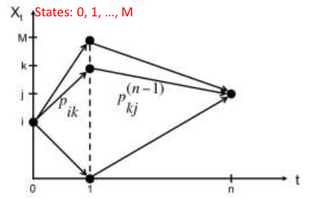
Example - Weather Forecasting, a two-state Markov chain: #
$$ P=\left[\begin{array}{ll} \alpha & 1-\alpha \\ \beta & 1-\beta \end{array}\right] $$If $\alpha = 0.7$ and $\beta = 0.4$, what is the probability that it will rain four days from today given that it is raining today?
The one-step transition probability matrix is given by
$$ P=\left|\begin{array}{ll} 0.7 & 0.3 \\ 0.4 & 0.6 \end{array}\right| $$Hence
$$ \begin{aligned} P^{(2)}=P^{2} &=\left|\begin{array}{ll} 0.7 & 0.3 \\ 0.4 & 0.6 \end{array}\right| \cdot\left|\begin{array}{ll} 0.7 & 0.3 \\ 0.4 & 0.6 \end{array}\right| \\ &=\left|\begin{array}{ll} 0.61 & 0.39 \\ 0.52 & 0.48 \end{array}\right| \end{aligned} $$$$ \begin{aligned} P^{(4)}=\left(P^{2}\right)^{2} &=\left|\begin{array}{ll} 0.61 & 0.39 \\ 0.52 & 0.48 \end{array}\right| \cdot\left|\begin{array}{ll} 0.61 & 0.39 \\ 0.52 & 0.48 \end{array}\right| \\ &=\left|\begin{array}{ll} 0.5749 & 0.4251 \\ 0.5668 & 0.4332 \end{array}\right| \end{aligned} $$The desired probability $P_{00}^{(4)} = 0.5749$
Example - Transforming a (non-Markov) Process into a Markov Chain (cont.) Given that it rained on Monday and Tuesday, what is the probability that it will rain on Thursday? #
The two-step transition matrix is given by
$$ \begin{aligned} P^{(2)}=P^{2} &=\left[\begin{array}{llll} 0.7 & 0 & 0.3 & 0 \\ 0.5 & 0 & 0.5 & 0 \\ 0 & 0.4 & 0 & 0.6 \\ 0 & 0.2 & 0 & 0.8 \end{array}\right] \cdot\left[\begin{array}{llll} 0.7 & 0 & 0.3 & 0 \\ 0.5 & 0 & 0.5 & 0 \\ 0 & 0.4 & 0 & 0.6 \\ 0 & 0.2 & 0 & 0.8 \end{array}\right] \\ &=\left[\begin{array}{llll} 0.49 & 0.12 & 0.21 & 0.18 \\ 0.35 & 0.20 & 0.15 & 0.30 \\ 0.20 & 0.12 & 0.20 & 0.48 \\ 0.10 & 0.16 & 0.10 & 0.64 \end{array}\right] \end{aligned} $$“Rain on Thursday” is equivalent to the process being in either state 0 or state 1 on Thursday. The desired probability is given by $P_{00}^{2}+P_{01}^{2}=0.49 + 0.12=0.61$.
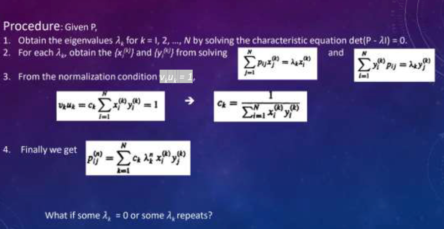
SOLVING FOR P(N) #
$$ PU = U\Lambda $$where $U \triangleq[u_1,u_2,\cdots,u_N]$ and
$$ \Lambda \triangleq\left(\begin{array}{llll} \lambda_1 & \lambda_2 & & 0 \\ 0 & \ddots & \lambda_N \end{array}\right) $$$U$ is non-singular(full rank and not zero determinant), $V = U^{-1}$ exists
$$ V \triangleq U^{-1}=\left[\begin{array}{c} v_1 \\ v_2 \\ \vdots \\ v_N \end{array}\right] $$Finally we can get
$$ P^{n}=U\Lambda^{n}V=\sum_{k = 1}^{N} \lambda_k^{n} u_k v_k^T $$or
$$p_{ij}^{(n)}=\sum_{k = 1}^{N}\lambda_{k}^{n}u_{ki}v_{kj}$$The calculation process #
EXAMPLE – EIGENVALUES AND EIGENVECTORS #
- Calculating Eigenvalues:
Given a matrix $A$, we calculate its eigenvalues by solving the characteristic equation $c(\lambda)=\text{det}(A - \lambda I_{2})$. For $A=\begin{bmatrix}1&1\ - 2&4\end{bmatrix}$, we have:
$$c(\lambda)=\text{det}\begin{pmatrix}\begin{bmatrix}1-\lambda&1\\ - 2&4-\lambda\end{bmatrix}\end{pmatrix}=(1 - \lambda)(4 - \lambda)+2 $$Expand the expression: $(1 - \lambda)(4 - \lambda)+2 = 4-\lambda - 4\lambda+\lambda^{2}+2=\lambda^{2}-5\lambda + 6$, set $\lambda^{2}-5\lambda + 6 = 0$. Factoring gives $(\lambda - 3)(\lambda - 2)=0$, so $\lambda_{1}=3$ and $\lambda_{2}=2$.
- Finding Eigenvectors:
- For $\lambda_{1}=3$:
- We solve the system $(A - 3I_{2})x = 0$. Here, $A - 3I_{2}=\begin{bmatrix}1 - 3&1\ - 2&4 - 3\end{bmatrix}=\begin{bmatrix}-2&1\ - 2&1\end{bmatrix}$.
- The augmented matrix is $\begin{bmatrix}-2&1&0\ - 2&1&0\end{bmatrix}$, which row - reduces to $$ \begin{bmatrix}1&-\frac{1}{2}&0\\0&0&0\end{bmatrix} $$ Let $$ x=\begin{bmatrix}x_{1}\\x_{2}\end{bmatrix} $$ , then $x_{1}=\frac{1}{2}x_{2}$, so $$ x = x_{2}\begin{bmatrix}\frac{1}{2}\\1\end{bmatrix} $$ Choosing $x_{2}=2$, we get the eigenvector $$ x=\begin{bmatrix}1\\2\end{bmatrix} $$
- For $\lambda_{2}=2$:
- We solve the system $(A - 2I_{2})x = 0$. Here, $A - 2I_{2}=\begin{bmatrix}1 - 2&1\ - 2&4 - 2\end{bmatrix}=\begin{bmatrix}-1&1\ - 2&2\end{bmatrix}$.
- The augmented matrix is $\begin{bmatrix}-1&1&0\ - 2&2&0\end{bmatrix}$, which row - reduces to $$ \begin{bmatrix}1&-1&0\\0&0&0\end{bmatrix} $$ Let $$ x=\begin{bmatrix}x_{1}\\x_{2}\end{bmatrix} $$ , then $x_{1}=x_{2}$, so $$ x = x_{2}\begin{bmatrix}1\\1\end{bmatrix} $$ Choosing $x_{2}=1$, we get the eigenvector $$ x=\begin{bmatrix}1\\1\end{bmatrix} $$
Example - BINARY COMMUNICATION CHANNEL #
- Calculating Eigenvalues of the Binary Communication Channel Matrix:
Given the binary communication channel matrix $P=\begin{bmatrix}1-\alpha&\alpha\\beta&1 - \beta\end{bmatrix}$, we find its eigenvalues by solving $\text{det}(P-\lambda I)=0$.
$\text{det}(P-\lambda I)=\begin{vmatrix}1-\alpha-\lambda&\alpha\\beta&1 - \beta-\lambda\end{vmatrix}=(1-\alpha-\lambda)(1 - \beta-\lambda)-\alpha\beta$.
Expand: $1-\beta-\lambda-\alpha+\alpha\beta+\alpha\lambda-\lambda+\lambda\beta+\lambda^{2}-\alpha\beta=\lambda^{2}-\lambda(2-\alpha-\beta)+(1-\alpha-\beta)=0$.
$\lambda_1 = 1$ and $\lambda_2 = 1-\alpha-\beta < 1$
- Finding Matrices U and V:
After solving for $U$ and $V$ and normalizing, we get
$$ U=\begin{bmatrix}1&-\alpha\\1&\beta\end{bmatrix} $$and
$$ V=\frac{1}{\alpha+\beta}\begin{bmatrix}\beta&\alpha\\ - 1&1\end{bmatrix} $$3. Calculating the \(n\)-step Transition Probability Matrix:
$$ P^{n}=\frac{1}{\alpha+\beta}\begin{bmatrix}1\\1\end{bmatrix}(\beta,\alpha)+\frac{(1-\alpha-\beta)^{n}}{\alpha+\beta}\begin{bmatrix}-\alpha\\\beta\end{bmatrix}(-1,1) $$- Expand further: $$ P^{n}=\frac{1}{\alpha+\beta}\begin{bmatrix}\beta&\alpha\\\beta&\alpha\end{bmatrix}+\frac{(1-\alpha-\beta)^{n}}{\alpha+\beta}\begin{bmatrix}\alpha&-\alpha\\-\beta&\beta\end{bmatrix} $$
- Calculating Conditional Probabilities:
- For example, to find $P(x_{0}=1|x_{n}=1)$:
- $P(x_{0}=1|x_{n}=1)=\frac{P{x_{0}=1|x_{0}=1}P(x_{0}=1)}{P(x_{n}=1)}=\frac{p_{11}^{(n)}p}{p_{11}^{(n)}p + p_{01}^{(n)}q}$.
- Substitute $p_{11}^{(n)}$ and $p_{01}^{(n)}$ from $P^{n}$: $P(x_{0}=1|x_{n}=1)=\frac{[\alpha+(1-\alpha-\beta)^{n}\beta]p}{\alpha+(1-\alpha-\beta)^{n}(\beta p-\alpha q)}$.
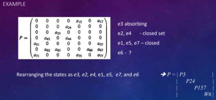
CLOSED SETS #
- Definition of a Closed Set:
- A set of states $C$ is closed if no state outside $C$ can be reached from any state in $C$.
- In a random walk with absorbing barrier, if $C$ is a closed set and $e_{i}\in C$, $e_{j}\notin C$, then $p_{ij}=0$ and $p_{ij}(n)=0$ for $n\geq1$.
- Absorbing State:
- A closed set with only one state is an absorbing state. If $e_{i}$ is an absorbing state, then $p_{ii}=1$ and $p_{ij}=0$ for $j\neq i$.
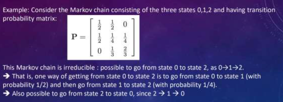
IRREDUCIBLE MARKOV CHAIN #
- Accessibility and Communication:
- State $e_{j}$ is accessible from state $e_{i}$ if $p_{ij}(n)>0$ for some $n$.
- If $e_{i}$ and $e_{j}$ are accessible from each other, they communicate.
- A Markov chain is irreducible if every state is accessible from every other state. Equivalently, a Markov chain is irreducible if there exists no closed set other than the set of all states.
- Example:
- In a simple random walk, every state can be reached from every other state, so it is an irreducible chain. Also, a binary communication channel is irreducible.
PERSISTENT (RECURRENT) STATE #
- First Passage Probability:
Define $f_{ij}^{(n)} = P[x_{n}=e_{j},x_{m}\neq e_{j},0 < m < n|x_{0}=e_{i}]$, the first passage probability from $e_{i}$ to $e_{j}$ in $n$ steps.
We have $p_{ij}^{(n)}=\sum_{r = 1}^{n}f_{ij}^{(r)}p_{jj}^{(n - r)}$ for $n\geq1$(not must be the first time)
Let $P(z)=\sum_{n = 0}^{\infty}p_{ij}^{(n)}z^{n}$ and $F(z)=\sum_{n = 1}^{\infty}f_{ij}^{(n)}z^{n}$
then we have $P_{ij}(z)=p_{ij}^{(0)}+F_{ij}(z)P_{jj}(z)$.
For $i = j$, $P_{ii}(z)=\frac{1}{1 - F_{ii}(z)}$. and $f_{ij}=\sum_{n = 1}^{\infty}f_{ij}^{(n)}=F_{ij}(1)$(first passage probability)
Classification of States:
- State $e_{i}$ is persistent (recurrent) if $f_{ii}=1$, start from $e_{i}$ and will return to $e_{i}$ with probability 1.
- A persistent state $e_{i}$ is null state if its mean recurrence time $\mu_{i}=\sum_{n = 1}^{\infty}nf_{ii}^{(n)}=\infty$, and non-null if $\mu_{i}<\infty$.
- State $e_{i}$ is transient if $f_{ii}<1$.
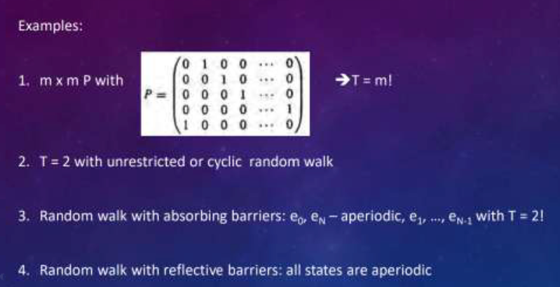
periodicity #
Definition of Period #
The period $T$ of a state is the greatest common divisor (gcd) of ${n:p_{ii}(n)<>0}$. All the none-zero $p_{ii}(n)$ and get the gcd.(the $p_{ii}(n)$ is the diagonal line elements).
State $i$ is periodic with period $T$ iff $p_{ii}(n)>0$ only when $n$ is a multiple of $T$.
If $T = 1$, the state is aperiodic.
Examples #
For
$$ P=\begin{bmatrix}0&1\\0.5&0.5\end{bmatrix} $$$P^1_{11}=0$, $P^2_{11}=0.5>0$, $P^3_{11}=0.25>0$, $\text{gcd}(2,3,\cdots)=1$, so state 1 is aperiodic, and state 2 is also aperiodic because 1 and 2 are communicated.
For
$$ P=\begin{bmatrix}0&1\\1&0\end{bmatrix} $$, $P^{2n + 1}_{11}=0$ and $P^{2n}_{11}=1$ for $n = 1,2,\cdots$, $\text{gcd}(2,4,\cdots)=2$, so state 1 has period 2.
Positive Recurrence AND Ergodicity #
- Positive Recurrence:
- State $i$ is positive recurrent when the expected value of the return time $T_{i}=\min\{n>0:X_{n}=i|X_{0}=i\}$ is finite, i.e., $E[T_{i}|x_{0}=i]=\sum_{n = 1}^{\infty}nP(T_{i}=n|x_{0}=i)<\infty$.
- Positive and null recurrence are class properties. Recurrent states in a finite - state MC are positive recurrent.
- Ergodicity:
- Jointly positive recurrent and aperiodic states are ergodic.
- An irreducible MC with ergodic states is an ergodic MC.
Examples #
KEY FACTS FOR A MARKOV CHAIN #
- A transient state will only be visited a finite number of times.
- In a finite-state Markov chain, at least one state must be persistent (not all states can be transient). because if all states are transient, the chain will not converge to a steady state.
- If state $i$ is persistent and state $i$ communicates with state $j$, then state $j$ is persistent.
- If state $i$ is transient and state $i$ communicates with state $j$, then state $j$ is transient.
- All states in a finite irreducible Markov chain are persistent., which can be reduced from the previous facts.
- A class of states is persistent if all states in the class are persistent, and transient if all states in the class are transient.
Examples #
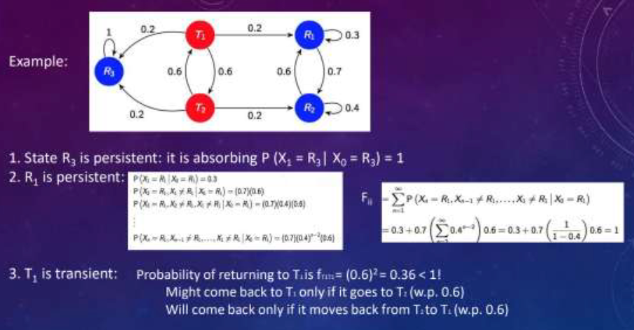
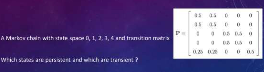
- For the state 0 and 1:
- From state 0, $p_{00} = 0.5$ and $p_{01}=0.5$; from state 1, $p_{10} = 0.5$ and $p_{11}=0.5$. This means that state 0 and 1 can transfer to each other, and they cannot transfer to states 2, 3, or 4. so ${0,1}$ forms a closed set.
- For the state 2 and 3:
- From state 2, $p_{22}=0.5$ and $p_{23}=0.5$; from state 3, $p_{32}=0.5$ and $p_{33}=0.5$. State 2 and 3 can transfer to each other, and they cannot transfer to states 0, 1, or 4. so ${2,3}$ forms a closed set.
- For the state 4:
- From state 4, $p_{40}=0.25$,$p_{41}=0.25$,$p_{42}=0.5$,it can transfer to other states, but there is no other state can transfer to it (the transfer probability from other states to state 4 is 0).
According to the definition of persistent and transient states, we can judge
- Persistent state (persistent state):
- If a state is in a closed set, then it is a persistent state. Because from the state in the closed set, it will not leave the set, and it will eventually return to the state (probability is \(1\)). So states \(0\), \(1\), \(2\), and \(3\) are persistent states.
- Transient state (transient state):
- State \(4\) is not a part of the closed set, from state \(4\), after a finite number of steps, it will enter the closed set \(\{0,1\}\) or \(\{2,3\}\), once it enters the closed set, it will not return to state \(4\), so state \(4\) is a transient state.
In conclusion, states \(0\), \(1\), \(2\), and \(3\) are persistent states, and state \(4\) is a transient state.
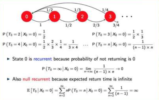
ONE-DIMENSIONAL RANDOM WALK #
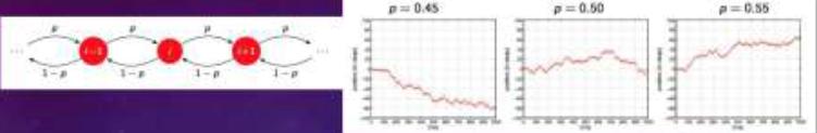
Transition Probabilities:
For a one-dimensional random walk with
$$ p_{j}=\begin{cases}p&j = i + 1\\1 - p&j = i - 1\\0&otherwise\end{cases} $$, for any state $e_{i}$,
$$ p_{ii}^{(n)}=\begin{cases}u_{2k}&n = 2k\\0&n = 2k+1\end{cases} $$, with $u_{2n}=\binom{2n}{n}(pq)^{n}$.
All states are periodic with period 2.
Look at the image:
- If $p\neq q$, $4pq<1$, $\sum_{i = 0}^{\infty}p_{ii}^{(2)}<\infty$ for every $e_{i}$, all states are transient.
- If $p = q$ ($4pq = 1$), the series diverges and every state is persistent.
2-D RANDOM WALK #
State Accessibility and Periodicity:
- The particle moves in unit steps in \(x\) and \(y\) directions independently. Every state is accessible from every other state, and all states are periodic with period 2.
- The particle can return to the origin when the positive steps and negative steps are the same.
Return Probability:
- n is the total steps of x y and k is the positive x.
- $p_{ii}^{(2n)}=\sum_{k = 0}^{n}\frac{2n!}{k!k!(n - k)!(n - k)!}(\frac{1}{2})^{4n}$. Using the approximation $\binom{2n}{n}\simeq\frac{\sqrt{4\pi n}(2n)^{2n}e^{-2n}}{(\sqrt{2\pi n}n^{n}e^{-n})^{2}}$, we get $p_{ii}^{(2n)}\simeq\frac{1}{\pi n}$ as $n\rightarrow\infty$.
- The series diverges, so all states are persistent null with periodicity 2.
3 - D RANDOM WALK #
State Accessibility and Periodicity:
- The particle moves independently in one of six directions. Every state is accessible from every other state and all states are periodic with period 2.
Return Probability:
$$ p_{ii}^{(2n)}\simeq P\{s_{2n}^{(x)}=0\}P\{s_{2n}^{(y)}=0\}P\{s_{2n}^{(z)}=0\}=\left\{\binom{2n}{n}2^{-2n}\right\}^{3}\simeq\frac{1}{\pi^{3/2}n^{3/2}} $$as $n\rightarrow\infty$.
- The series converges, so all states are transient. After some steps will never return to the origin.(the probability < 1)
STATIONARY DISTRIBUTIONS #
Existence of Limiting Distribution:
- every persistent state belongs to an irreducible closed set C containing similar states. Since no exit from C is ever possible.
- In an irreducible ergodic chain, the limits $q_{k}=\lim_{n\rightarrow\infty}p_{jk}^{(n)}>0$ exist independent of the initial state $e_{j}$. These limiting probabilities satisfy $q_{j}=\sum_{i}q_{i}p_{ij}$.
- Conversely, if a chain is irreducible and aperiodic and there exist non - negative numbers $q_{j}$ satisfying the above equations, then the chain is ergodic, and $q_{k}=\frac{1}{\mu_{k}}>0$, where $\mu_{j}$ is the mean recurrence time for the persistent non-null state $e_{j}$.
- If $e_{j}$ is either a transient state or a persistent null state, then $q_{j}=0$.
Example #
Consider the weather forecast as a two-state Markov chain. if $\alpha = 0.7$ and $\beta = 0.4$, then calculate the probability that it will rain four days from today given that it is raining today.
$$ P=\begin{bmatrix} 0.7 & 0.3 \\ 0.4 & 0.6 \end{bmatrix} $$Hence
$$ P^{(1)} = P=\begin{bmatrix} 0.7 & 0.3 \\ 0.4 & 0.6 \end{bmatrix} $$$$ P^{(2)}=P^{2}=\begin{bmatrix} 0.7 & 0.3 \\ 0.4 & 0.6 \end{bmatrix}\begin{bmatrix} 0.7 & 0.3 \\ 0.4 & 0.6 \end{bmatrix}=\begin{bmatrix} 0.61 & 0.39 \\ 0.52 & 0.48 \end{bmatrix} $$$$ P^{(4)} = P^{4}=(P^{2})^{2}=\begin{bmatrix} 0.61 & 0.39 \\ 0.52 & 0.48 \end{bmatrix}\begin{bmatrix} 0.61 & 0.39 \\ 0.52 & 0.48 \end{bmatrix}=\begin{bmatrix} 0.5769 & 0.4231 \\ 0.5683 & 0.4332 \end{bmatrix} $$$P^{(4)}$ is the desired probability that it will rain four days from today given that it is raining today.
$$ P^{(8)}=\left[\begin{array}{ll} 0.572 & 0.428 \\ 0.570 & 0.430 \end{array}\right] $$Note:
- $P^{(8)}$ is almost identical to $P^{(4)}$
- Each of the rows of $P^{(8)}$ has almost identical entries
STEADY - STATE MATRIX #
Convergence of Transition Probabilities
- For an ergodic (irreducible, aperiodic and positive recurrent) Markov chain, $\lim_{n\rightarrow\infty}P_{ij}^{n}$ exists and is independent of $i$.
- Let $\pi_{j}=\lim_{n\rightarrow\infty}P_{ij}^{n}$, then $\pi_{j}$ is the unique non-negative solution to the system $\pi_{j}=\sum_{i = 0}^{K}\pi_{i}P_{ij}$ ($\pi P=\pi$ in matrix form) and $\sum_{j = 0}^{K}\pi_{j}=1$.
This set of equations can be expanded as
$$ \begin{array}{r} \pi_{0} P_{00}+\pi_{1} P_{10}+\pi_{2} P_{20}+...+\pi_{K} P_{K 0}=\pi_{0} \\ \pi_{0} P_{01}+\pi_{1} P_{11}+\pi_{2} P_{21}+...+\pi_{K} P_{K 1}=\pi_{1} \\ \vdots \\ \pi_{0} P_{0 K}+\pi_{1} P_{1 K}+\pi_{2} P_{2 K}+...+\pi_{K} P_{K}=\pi_{K} \\ \pi_{0}+\pi_{1}+\pi_{2}+...+\pi_{K}=1 \end{array} $$Note:
$$\begin{aligned} P_{k j}^{n+1} & =\sum_{i=0}^{\infty} P\left(X_{n+1}=j | X_{n}=i, X_{0}=k\right) P_{k}^{n} \\ & =\sum_{i=0}^{\infty} P_{i j} P_{k i}^{n} \end{aligned} $$If the limits exists, for sufficiently large n
$$ \pi_{j}=\sum_{i=0}^{\infty} \pi_{i} P_{i j} $$Interpretation of Limiting Probability
The limiting probability $\pi_{j}$ that the process will be in state $j$ at time $n$ also equals the long-run proportion of time that the process will be in state $j$.
Consider the probability that the process will be in state j at time n +1
$$ P\left(X_{n+1}=j\right)=\sum_{i=0}^{\infty} P\left(X_{n+1}=j | X_{n}=i\right) P\left(X_{n}=i\right)=\sum_{i=0}^{\infty} P_{i j} P\left(X_{n}=i\right) $$Now,if we let n $\rightarrow\infty$,the result follows.
VECTOR/MATRIX NOTATION: MATRIX LIMIT #
For a finite-state Markov chain, $\lim_{n\rightarrow\infty}P^{n}=\begin{bmatrix}\pi_{1}&\pi_{2}&\cdots&\pi_{J}\\pi_{1}&\pi_{2}&\cdots&\pi_{J}\\vdots&\vdots&\ddots&\vdots\\pi_{1}&\pi_{2}&\cdots&\pi_{J}\end{bmatrix}$, where $\pi_{j}$ is the limiting probability of being in state $j$.
- Same probabilities for all rows ==> Independent of initial state
- $\lim_{n\rightarrow\infty}p(n)=\lim_{n\rightarrow\infty}(P^{T})^{n}p(0)=[\pi_{1},\cdots,\pi_{J}]^{T}$, which is independent of initial condition $p(0)$.
VECTOR/MATRIX NOTATION: EIGENVECTOR #
The vector limit (steady-state) distribution is $\boldsymbol{\pi}=[\pi_1,\pi_2,\cdots,\pi_J]$.
The limit distribution is the unique solution of $\boldsymbol{\pi}P^{T} = \boldsymbol{\pi}$ and $\boldsymbol{\pi}^{T}\mathbf{1}=1$, where $\mathbf{1}=(1,1,\cdots,1)^{T}$.
$\boldsymbol{\pi}$ is the eigenvector associated with eigenvalue 1 of $P^{T}$.
Eigenvectors are defined up to a scaling factor, and we normalize them to sum to 1. All other eigenvalues of $P$ have modulus smaller than 1. If not, $P^{n}$ diverges, but we know $P^{n}$ contains $n$-step transition probabilities. So, $\boldsymbol{\pi}$ is the eigenvector associated with the largest eigenvalue of $P$. Computing it as an eigenvector is often computationally efficient.
Example: Weather forecast again #
$$ P=\begin{bmatrix} \alpha & 1-\alpha \\ \beta & 1-\beta \end{bmatrix} $$If we say that the state is 0(whose limit prob is $\pi_{0}$) when it rains and 1 when it does not rain (the limiting probability $\pi_{1}$). We can deduce:
$$ \pi_{0}=\alpha \pi_{0}+\beta \pi_{1} $$$$ \pi_{1}=(1-\alpha) \pi_{0}+(1-\beta) \pi_{1} $$$$ \pi_{0}=\frac{\beta}{1+\beta-\alpha} \quad \pi_{1}=\frac{1-\alpha}{1+\beta-\alpha} $$$$ \pi_{0}+\pi_{1}=1 $$For example, if $\alpha = 0.7$ and $\beta = 0.4$, then the limiting probability of rain is $\pi_{0}=\frac{0.4}{1 + 0.4 - 0.7}=0.57$.
Example #
Does $P$ correspond to an ergodic MC?
$$ P=\begin{bmatrix} 0 & 0.3 & 0.7 \\ 0.1 & 0.5 & 0.4 \\ 0.1 & 0.2 & 0.7 \end{bmatrix} $$- Irreducible: all states communicate with state 2.
- positive recurrent, irreducible, and finite.
- It is also aperiodic since the period of state 2 is 1.
- There exist $\pi_{1}$, $\pi_{2}$, and $\pi_{3}$ such that $\pi_{j}=\lim_{n\rightarrow\infty}P_{ij}^{n}$ independent of $i$.
We solve the system of linear equations
$$ \pi_{j}=\sum_{i = 1}^{3}\pi_{i}P_{ij}\quad\text{and}\quad\sum_{j = 1}^{3}\pi_{j}=1 $$$$ \begin{bmatrix} \pi_{1} \\ \pi_{2} \\ \pi_{3} \\ 1 \end{bmatrix}=\begin{bmatrix} 0 & 0.1 & 0.1 \\ 0.3 & 0.5 & 0.2 \\ 0.7 & 0.4 & 0.7 \\ 1 & 1 & 1 \end{bmatrix}\begin{bmatrix} \pi_{1} \\ \pi_{2} \\ \pi_{3} \end{bmatrix} $$There are three variables and four equations. Some equations might be linearly dependent.
Indeed, summing the first three equations: $\pi_{1}+\pi_{2}+\pi_{3}=\pi_{1}+\pi_{2}+\pi_{3}$
This is always true because the probabilities in rows of $P$ sum up to 1, which is a manifestation of the rank deficiency of $1 - P$.
The solution yields $\pi_{1}=0.0909$, $\pi_{2}=0.2987$, and $\pi_{3}=0.6104$.
ERGODICITY #
The fraction of time $T_{i}^{(n)}$ spent in the $i$-th state by time $n$ is
$$ T_{i}^{(n)}:=\frac{1}{n}\sum_{m = 1}^{n}\mathbb{I}\{X_{m}=i\} $$The $\mathbb{I}{X_{m}=i}$ is an indicator function that is 1 if $X_{m}=i$ and 0 otherwise.
We compute the expected value of $T_{i}^{(n)}$:
$$ E\left[T_{i}^{(n)}\right]=\frac{1}{n}\sum_{m = 1}^{n}E\left[\mathbb{I}\{X_{m}=i\}\right]=\frac{1}{n}\sum_{m = 1}^{n}P\left(X_{m}=i\right) $$As $n\rightarrow\infty$, the probabilities $P(X_{m}=i)\rightarrow\pi_{i}$, so
$$ \lim_{n \to \infty}E\left[T_{i}^{(n)}\right]=\lim_{n \to \infty}\frac{1}{n}\sum_{m = 1}^{n}P\left(X_{m}=i\right)=\pi_{i} $$For ergodic Markov chains, the following holds without taking the expected value (almost surely a.s.):
$$ \lim_{n \to \infty}T_{i}^{(n)}=\lim_{n \to \infty}\frac{1}{n}\sum_{m = 1}^{n}\mathbb{I}\{X_{m}=i\}=\pi_{i} $$Example #
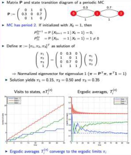
$$ P:=\begin{bmatrix} 0 & 0.3 & 0.7 \\ 0.1 & 0.5 & 0.4 \\ 0.1 & 0.2 & 0.7 \end{bmatrix} $$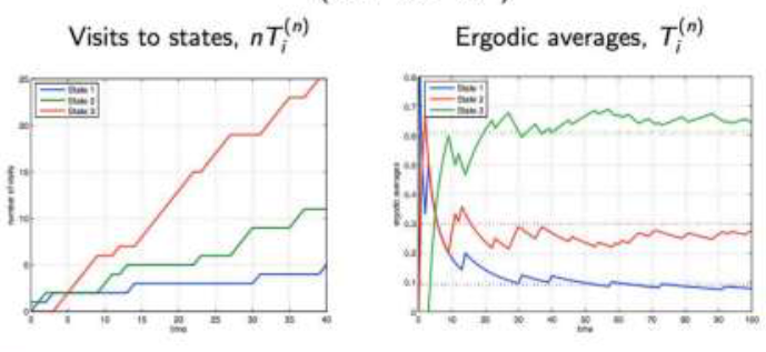
The visits to states $nT_{i}^{(n)}$ are ergodic averages. These ergodic averages slowly converge to $\boldsymbol{\pi}=[0.09,0.29,0.61]^{\top}$.
FUNCTION’S ERGODIC AVERAGE #
Consider an ergodic Markov chain with states $x_{n}=0,1,2,\cdots$ and stationary probabilities $\boldsymbol{\pi}$. Let $f(X_{n})$ be a bounded function of the state. Then,
$$ \lim_{n \to \infty}\frac{1}{n}\sum_{m = 1}^{n}f\left(X_{m}\right)=\sum_{j = 1}^{\infty}f(j)\pi_{j},\quad \text{a.s.} $$The ergodic average is equivalent to the expectation under the stationary distribution.
The use of ergodic averages is more general than $T_{i}^{(n)}$(the time propotion), and $T_{i}^{(n)}$ is a special case with $f(X_{m})=\mathbb{I}(X_{m}=i)$.
Think of $f(X_{n})$ as a reward (or cost) associated with the state. Then $\overline{f_{n}}=(1 / n)\sum_{m = 1}^{n}f(X_{m})$ is the time average of rewards (costs).
ERGODICITY IN PERIODIC MARKOV CHAINS #
Ergodic averages still converge if the Markov chain is periodic.
For an irreducible, positive recurrent Markov chain (periodic or aperiodic), we define
$$ \pi_{j}=\sum_{i = 0}^{\infty}\pi_{i}P_{i j},\quad\sum_{j = 0}^{\infty}\pi_{j}=1 $$- Claim 1: A unique solution exists (we say $\pi_{j}$ are well - defined).
- Claim 2: The fraction of time spent in state $i$ converges to $$ \lim_{n \to \infty}T_{i}^{(n)}=\lim_{n \to \infty}\frac{1}{n}\sum_{m = 1}^{n}\mathbb{I}\{X_{m}=i\}\to\pi_{i} $$
If the Markov chain is periodic, the probabilities $p_{ij}^{n}$ oscillate. But the fraction of time spent in state $i$ converges to $\pi_{i}$.
Example An perlodic Irreducible Markov chain #
REDUCIBLE MARKOV CHAINS #
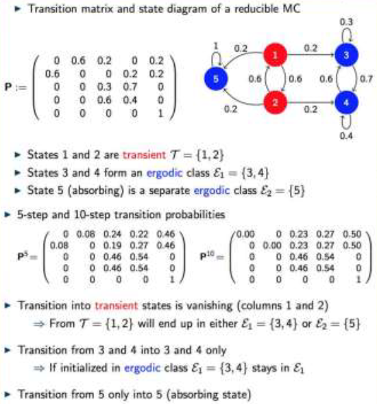
If a Markov chain is not irreducible, it can be decomposed into transient ($T$), ergodic ($E_{k}$), periodic ($P_{k}$), and null recurrent ($N_{k}$) components. All these are (communication) class properties.
the limit probabilities for transient states are null, i.e., $P(X_{n}=i)\to0$ for all $i\in T$.
For an arbitrary ergodic component $\epsilon_{k}$, we define conditional limits $\pi_{j}=\lim_{n \to \infty}P(X_{n}=j|X_{0}\in \epsilon_{k})$ for all $j\in \epsilon_{k}$. And $\pi_{j}$ satisfies
$$ \pi_{j}=\sum_{i\in \epsilon_{k}}\pi_{i}P_{i j},\quad\sum_{j\in \epsilon_{k}}\pi_{j}=1 $$For an arbitrary periodic component $P_{k}$, we re - define $\pi_{j}$ as
$$ \pi_{j}=\sum_{i\in P_{k}}\pi_{i}P_{i j},\quad\sum_{j\in P_{k}}\pi_{j}=1 $$
- The probabilities $P(X_{n}=j|X_{0}\in P_{k})$ do not converge (they oscillate).
- In addition, $$ \lim_{n \to \infty}T_{j}^{(n)}:=\lim_{n \to \infty}\frac{1}{n}\sum_{m = 1}^{n}\mathbb{I}\{x_{m}=i|X_{0}\in P_{k}\}\to\pi_{i} $$
- The limit probabilities for null-recurrent states are null, i.e., $P(X_{n}=i)\to0$ for all $i\in N$.
Example - Reducible Markov chain #

Related readings
If you want to follow my updates, or have a coffee chat with me, feel free to connect with me: