Markov Processes
April 20, 2025 · 8 min read · Page View:
If you have any questions, feel free to comment below. Click the block can copy the code.
And if you think it's helpful to you, just click on the ads which can support this site. Thanks!
This is a summary of the lecture notes of Markov Processes.
Outline #
- Markov Process
- Brownian Motion
- Wiener Process
- Geometric Brownian Motion
Stochastic Process #
A stochastic process is defined by:
- A collection of time points (index $t$).
- The state space, which are the possible values of $X_t$, e.g.,${11,12,\cdots,16, 21, 22,\cdots, 26,\cdots, 61, 62,\cdots 66}$, or the price $S_t$ of a stock at day $t$.
- The simultaneous distribution of the variables $X_t$, including the distributions of all $X_t$ and their dependencies.
There are two important types of processes:
- Poisson process: All variables are identically and independently distributed. Examples include tossing a coin/die, queues for counters, call centers, servers, etc.
- Markov process: The variables are dependent in a simple manner.
Markov Process #
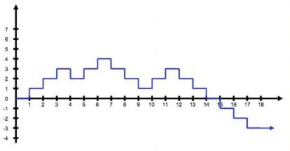
A 1st order Markov process in discrete time $(X_t),t = 1,\cdots$ satisfies the Markov Property:
$$ P(X_{t + 1}=x_{t + 1}|X_t=x_t,\cdots,X_1=x_1)=P(X_{t + 1}=x_{t + 1}|X_t=x_t) $$In other words, only the present state determines the future state; the past is irrelevant. The Markov property does not imply independence between $X_{t - 1}$ and $X_{t+1}$. In fact, often $P(X_{t+1}=x_{t+1}|X_{t-1}=x_{t-1})$ are not zero.
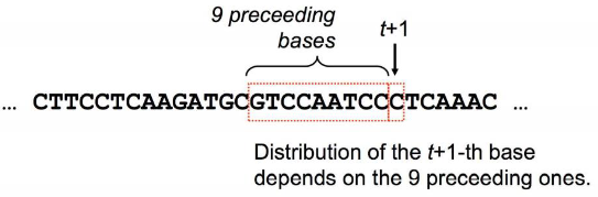
M-ORDER MARKOV PROCESS #
A stochastic process $(X_t),t = 1,2,\cdots$ with the property:
$$ P(X_{n + 1}=x_{n + 1}|X_n=x_n,\cdots,X_1=x_1)=P(X_{n + 1}=x_{n + 1}|X_n=x_n,\cdots,X_{n - m + 1}=x_{n - m + 1}) $$Loosely speaking, the future depends on the most recent past $m$ states.
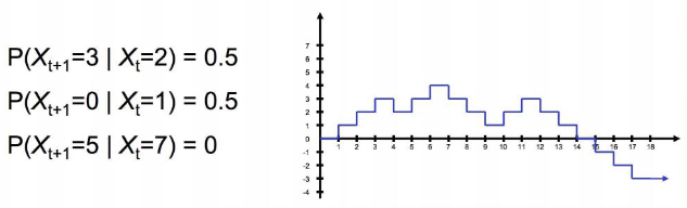
Transition Probabilities #
The transition probabilities are $P(X_{t+1}=x_{t + 1}|X_t=x_t)$ and $P(X_{t+1}=x_{t + 1}|X_s=x_s)$ for $s<t$.
Time Homogeneous Markov Process #
A Markov process is time homogeneous if the transition probabilities are independent of $t$:
$$ P(X_{t+1}=x_1 |X_t=x_2)=P(X_{s+1}=x_1|X_s=x_2) $$eg. $P(X_{584}=5 |X_{583}=4)=P(X_{213}=5|X_{212}=4)$
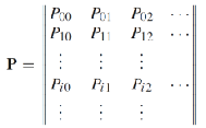
For a time-homogeneous Markov process with $N$ states, the one-step transition matrix $P=[p_{ij}]$, where $1\leq i,j\leq N$ and $p_{ij}=P(X_{t+1}=x_j|X_t=x_i)$ is independent of $t$.
$x_i$ is the state.
The initial distribution $(\pi_1,\cdots,\pi_N)$ gives the probabilities of the initial state, $\pi_i = P(X_1=x_i)$ for $i = 1,\cdots,N$ and $\sum_{i = 1}^{N}\pi_i=1$.
The $n$-step transition probabilities $p_{ij}^{(n)}=P(X_{t+n}=x_j|X_t=x_i)$.
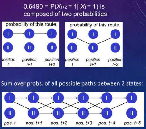
$$ p_{ij}^{(2)}=\sum_{k = 1}^{S}p_{kj}p_{ik}=\sum_{k = 1}^{S}p_{ik}p_{kj}=(p^{2})_{ij} $$$$ P^{(n)}=P^n, \text{for } n\geq2 $$Example: If
$$ P=\begin{pmatrix}0.35&0.65\\0.81&0.19\end{pmatrix} $$, then
$$ P^{(2)}=\begin{pmatrix}0.6490&0.3510\\0.4374&0.5626\end{pmatrix} $$and
$$ P^{(5)}=\begin{pmatrix}0.5456249&0.4543751\\0.5662212&0.4337788\end{pmatrix} $$eg. $p_{11}^{(2)} = p_{11}p_{11} + p_{12}p_{21}$ $= 0.35×0.35 + 0.65×0.81$ $= 0.1225 + 0.5265$ $= 0.6490$
We have known the start and end, then traverse(sum up) all possibilities in path.
KOLMOGOROV-CHAPMAN EQUATION #
Let $P_{ij}$ be the one - step transition probabilities and $P_{ij}^n$ be the $n$-step transition probabilities. For all $n,m\geq0$ and $i,j = 1,\cdots,S$:
$$ (P^{n + m})_{ij}=\sum_{k = 1}^{S}(P^{n})_{ik}(P^{m})_{kj} $$the probability that starting in state i the process will go to j in n + m transitions through a path which first takes it into state k at the nth transition,and then to state j in the next mth transition!
Wiener Process #
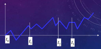
Consider a simple random walk ${X_N}$, where ${\xi_n}$ is a set of independent and identically distributed random variables with $P(\xi_k=\pm1)=\frac{1}{2}$. By the Central Limit Theorem, $\frac{X_N}{\sqrt{N}}\to N(0,1)$ in distribution.
Define a piecewise-constant random function $W_t^N=\frac{X_{\lfloor Nt\rfloor}}{\sqrt{N}}$ on $t\in[0,\infty)$.
As $N\to\infty$, $W^N$ converges in distribution to a stochastic process $W_t$ (or $W(t)$), which is the Wiener process.
A stochastic process $W(t)$ with values in $\mathbb{R}$ defined for $t\in[0,\infty)$ satisfies:
- $W(0)=0$.
- If $0<s<t$, then $W(t)-W(s)$ has a normal distribution $\sim N(0,t - s)$ with mean $0$ and variance $(t - s)$. :stationary
- If $0\leq s<t\leq u<v$, then $W(t)-W(s)$ and $W(v)-W(u)$ are independent random variables. :Gaussianity
- The sample paths $t\to W(t)$ are almost surely continuous.
In fact, the Wiener process is the only time-homogeneous stochastic process with independent increments that has continuous trajectories.
The probability density function of $W(t)$ is $f_{W(t)}(x)=\frac{1}{\sqrt{2\pi t}}e^{-\frac{x^2}{2t}}$.
Definition of Brownian Motion #
Brownian motion $B(t)$ is the unique process with the following properties:
- No memory: $B_{t_1}-B_{t_0},B_{t_2}-B_{t_1},B_{t_3}-B_{t_2},\cdots$ are independent.
- Invariance: The distribution of $B_{t + s}-B_s$ depends only on $t$.
- Continuity.
- $B_0 = 0$, $B_t - B_0 = B_t\sim N(0,t)$, $E(B_t)=0$, $Var(B_t)=t$.
Brownian motion is a Wiener process
Basic properties #
- Path regularity: $t\to B_t$ is continuous almost surely, but is nowhere differentiable almost surely. $dB(t)/dt \to \infty$
- $B_t$ is a Gaussian process. For all $0\leq t_1\leq\cdots\leq t_n$, the random vector $Z=(B_{t_1},\cdots,B_{t_n})$ has a multinormal distribution.
- $B_t$ has stationary increments: $(B_{t+h}-B_t)$ for $h>0$ has the same distribution for all $t$, $E(B_{t+h}-B_t)=0$ and $Var(B_{t+h}-B_t)=h$.
- Brownian motion is a martingale: $E(B_t|B_s)=B_s$ almost surely if $s<t$, where $F_s$ is the “information up to time $s$”. Which means, the expected value of $B_t$ at time $t$ is the value of $B_s$ at time $s$, the best prediction is now, which is related to the independent increments.
- $Cov(B_s,B_t)=\min(s,t)$
Local Extremes
- Brownian motion paths contain local maxima and minima in any non-trivial interval, making the set of local maxima and minima dense. This means that for any given number, there exists a local maximum or minimum arbitrarily close to it.
- Each local maximum and minimum is isolated, and the set of local maxima and minima is countable.
Increasing and Decreasing Points
- Define increasing and decreasing points: $\exists \epsilon > 0$ s.t. $\forall s \in (0, \epsilon)$, $f(t-s) \leq f(t) \leq f(t+s)$. Then $t$ is an increasing point (otherwise it is a decreasing point).
- But for standard Brownian motion, there are no pure increasing or decreasing points on any non-trivial interval. means the BM is not monotonic on any non-trivial interval.
Distributional Properties #
- Spatial Homogeneity: $B_t+x$ for any $x\in\mathbb{R}$ is a Brownian motion started at $x$.
- Symmetry: $-B_t$ is also a Brownian motion.
- Scaling: $cB_{\frac{t}{c^2}}$ for any $c>0$ is a Brownian motion.
- Time inversion: $Z_t=\begin{cases}0, & t = 0\tB_{\frac{1}{t}}, & t>0\end{cases}$
- Time reversibility: For any given $t>0$, ${B_s:0\leq s\leq t}\sim{B_{t - s}-B_t:0\leq s\leq t}$
Relatives of Brownian Motion #
- For $\mu\in\mathbb{R}$, $\sigma>0$, $x\in\mathbb{R}$, the process ${x+\mu t+\sigma W(t),t\geq0}$ is a Brownian motion with drift $\mu$ and diffusion coefficient $\sigma$ starting from $x$.
- For $Y_t = e^{x+\mu t+\sigma W(t)}$, the process $(Y_t,t\geq0)$ is a Geometric Brownian motion.
- For $B_t^0=W(t)-tW(1)$, the process $(B_t^0,t\geq0)$ is a Brownian bridge. normally used to model the stochastic process of fixed start and end.
Invariance Principle #
- Random walk converges to Brownian motion: ${\sqrt{a}W_{\frac{t}{a}},t\geq0}\stackrel{a\to\infty}{\to}{B_t,t\geq0}$
- Reflected random walk converges to reflected Brownian motion.
Why Brownian Motion? #
Brownian motion is unique:
- It is nowhere differentiable even though continuous everywhere.
- It is self-similar (fractal). The slices of BM also look like BM.
- It will eventually hit any real value. and return 0 again and again.
- It belongs to several families of stochastic processes, such as Markov processes, martingales, Gaussian processes, and Levy processes.
Brownian Motion for Financial Markets #
Financial markets (stock, foreign exchange, commodity, and bond markets) are often assumed to follow Brownian motion. A standard Brownian motion is insufficient for asset price movements and that a geometric Brownian motion is necessary.
Geometric Brownian Motion (GBM) #
Geometric Brownian Motion is the continuous-time stochastic process $X(t)=z_0e^{\mu t+\sigma W(t)}$, where $W(t)$ is a standard Brownian Motion. It is used as a simple model for market prices because it is always positive (with probability 1).
The relative change is given by $\frac{dX}{X}=\mu dt+\sigma dW$. A random variable $X$ has a log-normal distribution (with parameters $\mu$ and $\sigma$) if $\log(X)$ is normally distributed: $\log(X)\sim N(\mu,\sigma^2)$.
The probability density function of $X$ is:
$$ f_X(x)=\frac{1}{\sqrt{2\pi}\sigma x}\exp\left((-1/2)[(\ln(x)-\mu)/\sigma]^2\right) $$At fixed time $t$, $GBM$ $X(t)=z_0e^{\mu t+\sigma W(t)}$ has a log - normal distribution with parameters $(\ln(z_0)+\mu t)$ and $\sigma\sqrt{t}$.
$$ E[z_0\exp(\mu t+\sigma W(t))]=z_0\exp\left(\mu t+\frac{1}{2}\sigma^2t\right) $$$$ Var[z_0\exp(\mu t+\sigma W(t))]=z_0^2\exp(2\mu t+\sigma^2t)[\exp(\sigma^2t)-1] $$Reasonable Model for Stock Price-Geometric Brownian Motion #
The stock price $S$ can be modeled by $dS=\mu Sdt+\sigma Sdz$, where $\mu$ is the “expected return”, $\sigma$ is the “volatility”, and $Z$ is a Wiener process. Then $d\ln S=(\mu-\frac{\sigma^2}{2})dt+\sigma dz$.
The analytical solution $S = S_0e^{(\mu-\frac{\sigma^2}{2})t+\sigma Z}$.
$\ln S$ has $T$ - period changes that are normally distributed.
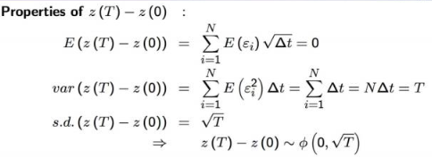
If $Z(t)$ is a Wiener process, for $dz\sim N(0, dt)$ = $N(0,1)\sqrt{dt}$ which $\Delta Z = Z(t+\Delta t)-Z(t)$:
$$ E(\Delta Z)=0 $$$$ Var(\Delta Z)=\Delta t $$$$ S.D.(\Delta Z)=\sqrt{\Delta t} $$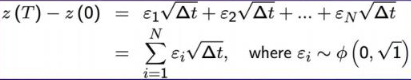
Some important things about WIENER PROCESS #
the Wiener process can be used to generate any continuous time stochastic process
Generalized Wiener Process $x$: a linear function of $z$ and time $dx =adt +bdz$, which $a dt$:deterministic component,or"drift"→$E(Ax)=at+bE(Az) =a t$,if $t=1$,then $E(△x)=a$!
For example, from time $0$ to $T$:
- $x(T)-x(0)=aT + b(z(T)-z(0))$ ,which is the change of $x$ in the time interval $[0, T]$.
- $E[x(T)-x(0)] = aT + bE[z(T)-z(0)] = aT$ ,the expected change of $x$ in the time interval $[0, T]$.
- $var[x(T)-x(0)] = b^{2}var[z(T)-z(0)] = b^{2}T$ ,the variance of the change of $x$ in the time interval $[0, T]$.
- $s.d.[x(T)-x(0)] = b\sqrt{T}$ ,the standard deviation of the change of $x$ in the time interval $[0, T]$.
- $x(T)-x(0)$ follows the normal distribution $N(aT,b\sqrt{T})$.
Consider the function $G(S,t)=\ln S$ , where $S$ is usually the stock price, and $t$ is time.
Ito’s Lemma provides a formula for differentiating a function of a stochastic process. For $dG = d\ln S$ , according to Ito’s Lemma formula $dG=\left(\frac{\partial G}{\partial S}\mu S+\frac{\partial G}{\partial t}+\frac{1}{2}\frac{\partial^{2}G}{\partial S^{2}}(\sigma S)^{2}\right)dt+\frac{\partial G}{\partial S}\sigma Sdz$ .
For $G(S,t)=\ln S$ , the partial derivatives are $\frac{\partial G}{\partial S}=\frac{1}{S}$ , $\frac{\partial G}{\partial t}=0$ , $\frac{\partial^{2}G}{\partial S^{2}}=-\frac{1}{S^{2}}$ . Substituting these partial derivatives into Ito’s Lemma formula:
$$ \begin{align*} dG&=\left[\frac{1}{S}\mu S + 0+\frac{1}{2}\left(-\frac{1}{S^{2}}\right)(\sigma S)^{2}\right]dt+\frac{1}{S}\sigma Sdz\\ &=\left(\mu-\frac{\sigma^{2}}{2}\right)dt+\sigma dz \end{align*} $$
So $\ln S$ is a generalized Wiener process. This conclusion makes it easier to analyze stock price-related analysis, as generalized Wiener processes have some good properties.
Stock Prices Are Log-Normally Distributed #
Since stocks follow the geometric brownian motion $dS=\mu Sdt+\sigma Sdz$, $\ln S$ follows the generalized Wiener Process $d\ln S=(\mu-\frac{\sigma^2}{2})dt+\sigma dz$. Assume $\mu\geq \sigma^2$, then:
$$ E(\ln S_T-\ln S_0)=(\mu-\frac{\sigma^2}{2})T $$$$ Var(\ln S_T-\ln S_0)=\sigma^2T $$$$ \ln S_T-\ln S_0\sim N((\mu-\frac{\sigma^2}{2})T,\sigma\sqrt{T}) $$or
$$ \ln S_T\sim N(\ln S_0+(\mu-\frac{\sigma^2}{2})T,\sigma\sqrt{T}) $$Predicting Stock Prices with a GBM Model #
let $S_0$ is current stock price, $S_N$ is the stock price at future time $N$($N=T/\Delta t$, if $\Delta t = 1$ means daily price).
- daily return: $r_k=\frac{S_k - S_{k - 1}}{S_{k - 1}}$ ($k$ is time period)
- average return: $\hat{\mu}=\frac{1}{M}\sum_{k = 1}^{M}r_k$ calculate average to estimate $\mu$ and
- use $\hat{\sigma}=\sqrt{\frac{1}{M}\sum_{k = 1}^{M}(r_k-\hat{\mu})^2}$ to estimate $\sigma$ 。
- drift: $drift_k=\mu-\frac{\sigma^{2}}{2}$ which means long term deterministic trend
- diffusion: $diffusion_k=\sigma b_k= \sigma z_k$ and $b_k\sim N(0,1)$, which means short term random fluctuation
- stock price: $S_{t_1}=S_{t_0}+S_{t_0}drift_{t_1}+S_{t_0}diffusion_{t_1}$ $$ \begin{align*} S_{k}&=S_{k - 1} \cdot e^{(drift_{k}+diffusion_{k})}=S_{k - 1} \cdot e^{\left(\mu-\frac{1}{2}\sigma^{2}+\sigma z_{k}\right)}\\ S_{k}&=S_{0} \cdot e^{\left(\left(\mu-\frac{1}{2}\sigma^{2}\right)t_{k}+\sigma W_{k}\right)}\\ t_{k}&=k\\ W_{k}&=\sum_{i = 1}^{k}b_{i} \text{ and } b_{i}\sim N(0,1) \end{align*} $$
Related readings
If you want to follow my updates, or have a coffee chat with me, feel free to connect with me: