Possion Processes

April 19, 2025 · 18 min read · Page View:

If you have any questions, feel free to comment below.

This article is mainly about the Poisson processes in the book “Random Processes” by Gregory F. Lawler.

Outline #

• Definition of Poisson Process
• Axiomatic Development
• Sum of Poisson Processes
• Inter-arrival Distribution for Poisson Processes
• Poisson Departures between Exponential Interarrivals
• Independent and stationary increments
• Bulk Arrivals and Compound Poisson Processes

Review of Some Basic Properties #

Poisson arrivals can be seen as the limiting behavior of Binomial random variables (refer to Poisson approximation of Binomial random variables).

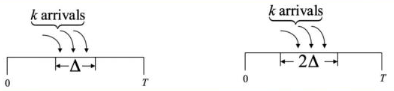
The probability that $k$ arrivals occur in an interval of duration $\Delta$ is given by

, where $\lambda=np=\mu T\cdot\frac{\Delta}{T}=\mu\Delta$.

For an interval of duration $2\Delta$,

, and $np_{1}=\mu T\cdot\frac{2\Delta}{T}=2\mu\Delta = 2\lambda$.

Poisson arrivals over an interval form a Poisson random variable whose parameter depends on the duration of that interval. Also, due to the Bernoulli nature of the underlying basic random arrivals, events over non-overlapping intervals are independent.

Example 9-5.

Definition of Poisson Process #

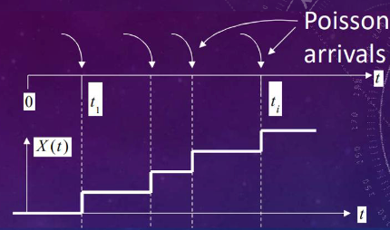
$X(t)=n(0, t)$ represents a Poisson process if:

1. The number of arrivals $n(t_{1}, t_{2})$ in an interval $(t_{1}, t_{2})$ of length $t=t_{2}-t_{1}$ is a Poisson random variable with parameter $\lambda t$, i.e., $P{n(t_{1}, t_{2}) = k}=e^{-\lambda t} \frac{(\lambda t)^{k}}{k!}, k = 0,1,2,\cdots$.
2. If the intervals $(t_{1}, t_{2})$ and $(t_{3}, t_{4})$ are non-overlapping, then the random variables $n(t_{1}, t_{2})$ and $n(t_{3}, t_{4})$ are independent.

Since $n(0, t)\sim P(\lambda t)$, we have:

• $E[X(t)] = E[n(0, t)]=\lambda t$
• $E[X^{2}(t)] = E[n^{2}(0, t)]=\lambda t+\lambda^{2}t^{2}$
  • Since $E[X(t)] = \lambda t$, $VAR[X(t)] = E[X(t)]$.

Autocorrelation Function $R_{XX}(t_{1}, t_{2})$ #

Let $t_{2}>t_{1}$. Then $n(0,t_{1})$ and $n(t_{1},t_{2})$ are independent Poisson random variables with parameters $\lambda t_{1}$ and $\lambda(t_{2}-t_{1})$ respectively.

So, $E\left[n\left(0, t_{1}\right) n\left(t_{1}, t_{2}\right)\right]=E\left[n\left(0, t_{1}\right)\right] E\left[n\left(t_{1}, t_{2}\right)\right]=\lambda^{2}t_{1}(t_{2}-t_{1})$.

Since $n(t_{1}, t_{2})=n(0, t_{2}) - n(0, t_{1})=X(t_{2}) - X(t_{1})$, we have

Therefore,

• $R_{XX}\left(t_{1}, t_{2}\right)=\lambda^{2}t_{1}(t_{2}-t_{1})+E\left[X^{2}\left(t_{1}\right)\right]=\lambda t_{1}+\lambda^{2}t_{1}t_{2}, t_{2}\geq t_{1}$.
• Similarly, $R_{XX}\left(t_{1}, t_{2}\right)=\lambda t_{2}+\lambda^{2}t_{1}t_{2}, t_{2}<t_{1}$.

In general, $R_{XX}\left(t_{1}, t_{2}\right)=\lambda^{2}t_{1}t_{2}+\lambda\min\left(t_{1}, t_{2}\right)$.

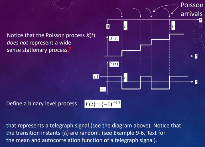
Binary Level Process and Stationarity

Define a binary level process $Y(t)=(-1)^{X(t)}$ representing a telegraph signal. The transition instants ${t}$ are random.

Although $X(t)$ is not a wide-sense stationary process, its derivative $X^{\prime}(t)$ is a wide-sense stationary process.

Thus nonstationary inputs to linear systems can lead to wide sense stationary outputs, an interesting observation.

Some Typical Poisson Processes #

• Arrivals to a queueing system.
• Earthquakes in a geological system.
• Accidents in a given city.
• Claims on an insurance company.
• Demands on an inventory system.
• Failures in a manufacturing system (e.g., an average of 1 failure per week, $P(X = 0 \text{ failures}) = 0.36788$, $P(X = 1 \text{ failure}) = 0.36788$, $P(X = 2 \text{ failures}) = 0.18394$).

Modeling is more tractable if the successive inter-event (inter-arrival) times are independent and identically-distributed (iid) exponential random variables, which leads to a Poisson process.

Example of Poisson Process Application #

Let $N(t)$ be the number of births in a hospital over the interval $(0, t)$ and assume $N(t)$ is a Poisson process with rate 10 per day.

1. For an 8-hour shift ($\frac{1}{3}$ day), $N(\frac{1}{3})\sim Poisson(\frac{10}{3})$. So, $E[N(\frac{1}{3})]=\frac{10}{3}$ and $Var[N(\frac{1}{3})]=\frac{10}{3}$.
2. For the probability that there are no births from noon to 1 p.m. (1 hour = $\frac{1}{24}$ day), $N(\frac{1}{24})\sim Poisson(\frac{10}{24})$. The probability $P[N(\frac{1}{24}) = 0]=e^{-\frac{10}{24}}\approx0.6592$.
3. For the probability that there are three births from 8 a.m. to 12 noon ($4$ hours = $\frac{4}{24}$ day) and four from 12 noon to 5 p.m. ($5$ hours = $\frac{5}{24}$ day), a

Assuming 8 a.m. is $t = 0$, the probability will be:

$P(N(\frac{12}{24})-N(\frac{8}{24})=3;N(\frac{17}{24})-N(\frac{12}{24}) = 4)=P(N(\frac{12}{24})-N(\frac{8}{24})=3)P(N(\frac{17}{24})-N(\frac{12}{24}) = 4)$ (by independence of increments) $=P(N(\frac{4}{24}) = 3)P(N(\frac{5}{24}) = 4)$ (by stationarity of increments) $=e^{-\frac{10}{6}}\frac{(\frac{10}{6})^{3}}{3!}e^{-\frac{10}{6}}\frac{(\frac{10}{6})^{4}}{4!}\approx0.0088$

Sum and Difference of Poisson Processes #

If $X_{1}(t)$ and $X_{2}(t)$ are two independent Poisson processes:

• Superposition/Sum: $X_{1}(t)+X_{2}(t)$ is also a Poisson process with parameter $(\lambda_{1}+\lambda_{2})t$.
• No Difference: $Y(t)=X_{1}(t)-X_{2}(t)$ is not a Poisson process since $E{y(t)}=(\lambda_{1}-\lambda_{2})t$ and $Var{y(t)}=(\lambda_{1}+\lambda_{2})t$.

Example of Sum of Poisson Processes #

Let $B(t)$ be the number of boys born in a hospital over $(0, t)$ with rate 10 per day and $G(t)$ be the number of girls born with rate 9 per day. They are independent Poisson processes.

Let $N(t)=B(t)+G(t)$. Then $N(t)$ is a Poisson process with rate $10 + 9 = 19$ per day.

Then mean and variance of $N(t)$ are $19t$ respectively, when t is a week, the value is $19\times7=133$.

Random Selection of Poisson Points #

Remember the random process definition? (t and $\xi$)

Let $t_{1}, t_{2},\cdots,t_{i},\cdots$ be random arrival points of a Poisson process $X(t)$ with parameter $\lambda t$. Define an independent Bernoulli random variable $N_{i}$ for each arrival point, where $P(N_{i}=1)=p$ and $P(N_{i}=0)=q = 1 - p$.

Define:

• $Y(t)=\sum_{i = 1}^{X(t)}N_{i}$, Each arrival of $X(t)$ gets tagged independently with probability $p$.
• $Z(t)=\sum_{i = 1}^{X(t)}(1 - N_{i})=X(t)-Y(t)$, Each arrival of $X(t)$ gets untagged independently with probability $q = 1 - p$.

Both $Y(t)$ and $Z(t)$ are independent Poisson processes with parameters $\lambda p t$ and $\lambda q t$ respectively.

Proof:

• Let $A_{n}={n \text{ events occur in }(0, t)\text{ and }k \text{ of them are tagged}}$.

$P(A_{n})=P{k \text{ events are tagged}|x(t)=n}P{x(t)=n}=\binom{n}{k}p^{k}q^{n - k}e^{-\lambda t}\frac{(\lambda t)^{n}}{n!}$

So the probability that $Y(t)=k$ is the sum of the probabilities that $n$ events occur in $(0, t)$ and $k$ of them are tagged for all $n\geq k$, ${Y(t)=k}=\bigcup_{n = k}^{\infty}A_{n}$.

$P{Y(t)=k}=\sum_{n = k}^{\infty}P{Y(t)=k|X(t)=n}P{X(t)=n}$

Since $P{Y(t)=k|X(t)=n}=\binom{n}{k}p^{k}q^{n - k}$ and $P{X(t)=n}=e^{-\lambda t}\frac{(\lambda t)^{n}}{n!}$, we have $P{Y(t)=k}=e^{-\lambda p t}\frac{(\lambda p t)^{k}}{k!}\sim P(\lambda p t)$.

In the end: $P{Y(t)=k,Z(t)=m}=P{Y(t)=k,X(t)-Y(t)=m}=P{Y(t)=k,X(t)=k + m}=P{Y(t)=k|X(t)=k + m}P{X(t)=k + m}=\binom{k + m}{k}p^{k}q^{m}e^{-\lambda t}\frac{(\lambda t)^{k + m}}{(k + m)!}=P{Y(t)=k}P{Z(t)=m}$

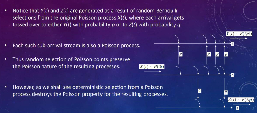
Thus random selection (not deterministic) of Poisson points preserve the Poisson nature of the resulting processes!

Example of Random Selection #

Let $N(t)$ be the number of births in a hospital with rate 16 per day, 48% of births are boys and 52% are girls.

Let $B(t)$ and $G(t)$ be the number of boys and girls born respectively. Then $B(t)\sim Poisson(16\times0.48)$ and $G(t)\sim Poisson(16\times0.52)$.

The probability that we see six boys and eight girls born on a given day is $P(B(1)=6,G(1)=8)=e^{-7.68}\frac{7.68^{6}}{6!}e^{-8.32}\frac{8.32^{8}}{8!}\approx0.0183$

Inter-arrival Distribution for Poisson Processes #

Let $\tau_{1}$ be the time interval to the first arrival from a fixed point $t_{0}$.

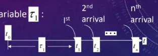
To determine the probability distribution of the random variable $\tau_{1}$:

The event ${\tau_{1}\leq t}$ is the same as ${n(t_{0}, t_{0}+t)>0}$, or ${\tau_{1} > t}$ is the same as ${n(t_{0}, t_{0}+t)=0}$.

So $F_{\tau_{1}}(t)=P{\tau_{1}\leq t}=P{X(t)>0}=1 - P{n(t_{0}, t_{0}+t)=0}=1 - e^{-\lambda t}$.

The probability density function $f_{\tau_{1}}(t)=\frac{dF_{\tau_{1}}(t)}{dt}=\lambda e^{-\lambda t},t\geq0$.

So $\tau_{1}$ is an exponential random variable with parameter $\lambda$ and $E(\tau_{1})=\frac{1}{\lambda}$.

All inter-arrival durations $\tau_{1},\tau_{2},\cdots,\tau_{n},\cdots$ of a Poisson process are independent exponential random variables with common parameter $\lambda$, i.e., $f_{\tau_{i}}(t)=\lambda e^{-\lambda t},t\geq0$.

Let $t_{n}$ be the $n^{th}$ random arrival point.

• Then $F_{t_{n}}(t)=P{t_{n}\leq t}=P{X(t)\geq n}=1 - P{X(t)<n}=1-\sum_{k = 0}^{n - 1}\frac{(\lambda t)^{k}}{k!}e^{-\lambda t}$.

• The probability density function $f_{t_{n}}(x)=\frac{dF_{t_{n}}(x)}{dx}=\frac{\lambda^{n}x^{n - 1}}{(n - 1)!}e^{-\lambda x},x\geq0$, which is a gamma density function.

The waiting time to the $n^{th}$ Poisson arrival instant has a gamma distribution, and $t_n=\sum_{i = 1}^{n}\tau_i$, $\tau_i$ means the inter-arrival time between the $(i-1)^{th}$ and $i^{th}$ Poisson arrival instant.

If we systematically tag every $m^{th}$ outcome of a Poisson process $X(t)$ to generate a new process $e(t)$, the inter - arrival time between any two events of $e(t)$ is a gamma random variable. If $\lambda=m\mu$, then $E[e(t)]=\frac{1}{\mu}$, and the inter-arrival time represents an Erlang-$m$ random variable, and $e(t)$ is an Erlang-$m$ process.

Conclusion #

In summary, if Poisson arrivals are randomly redirected to form new queues, then each such queue generates a new Poisson process.

However if the arrivals are systematically redirected (1st arrival to 1st counter, 2nd arrival to 2nd counter, $m^{th}$ arrival to $m^{th}$ counter, $(m +1)^{st}$ arrival to 1st counter), then the new subqueues form Erlang-$m$ processes.

Little O(H) Notation #

Let $o(h)$ denote any function of $h$ such that $\frac{o(h)}{h}\to0$ as $h\to0$, which can be ignored.

Examples:

1. $h^{k}$ is $o(h)$ for any $k > 1$ since $\frac{h^{k}}{h}=h^{k - 1}\to0$ when $h\to0$.
2. The finite series $\sum_{k = 2}^{\infty}c_{k}h^{k}$ with $|c_{k}|<1$ is $o(h)$ because $\lim_{h\to0}\frac{\sum_{k = 2}^{\infty}c_{k}h^{k}}{h}=\lim_{h\to0}\sum_{k = 2}^{\infty}c_{k}h^{k - 1}=0$. where taking the limit inside the summation is justified because the sum is bounded by 1 /（1 - h） for h <1.

• $o(h)+o(h)=o(h)$
• $o(h)o(h)=o(h)$
• $co(h)=o(h)$ for any constant $c$.
• even for any linear combination.

Axiomatic Development of Poisson Processes #

Some conditions:

The defining properties of a Poisson process are that in any “small” interval one event can occur with probability that is proportional to $\Delta t$.

Further, the probability that two or more events occur in that interval is proportional to $o(\Delta t)$, higher powers of $\Delta t$, and events over non-overlapping intervals are independent of each other.

This gives rise to the following Axioms:

1. $P{n(t, t+\Delta t)=1}=\lambda \Delta t+o(\Delta t)$: means only one event occurs in the interval.
2. $P{n(t, t+\Delta t)=0}=1-\lambda \Delta t+o(\Delta t)$ : means no event occurs in the interval.
3. $P{n(t, t+\Delta t) \geq 2}=o(\Delta t)$ : means two or more events occur in the interval.
4. $n(t, t+\Delta t)$ is independent of $n(0, t)$ : means the events are independent of each other.

Notice that axiom3 specifies that the events occur singly, and axiom4 specifies the randomness of the entire series. Axiom2 follows from 1 and 3 together with the axiom of total probability.

first arrival time interval #

Let $t_0$ be any fixed point and let $\tau_1$ represent the time of the first arrival after $t_0$. Notice that the random variable $\tau_1$ (Axiom4), is independent of the occurrences prior to the instant $t_0$. With $F_{\tau_{1}}(t)=P{\tau_{1} \leq t}$ representing the distribution function of $\tau_1$.

Now define $Q(t)=1 - F_{\tau_{1}}(t)=P{\tau_{1}>t}$. Then for $\Delta t>0$

$$ \begin{aligned} Q(t+\Delta t) &=P\left\{\tau_{1}>t+\Delta t\right\}\\ &=P\left\{\tau_{1}>t, \text{ and no event occurs in } \left(t_{0}+t, t_{0}+t+\Delta t\right)\right\}\\ &=P\left\{\tau_{1}>t, n\left(t_{0}+t, t_{0}+t+\Delta t\right)=0\right\}\\ &=P\left\{n\left(t_{0}+t, t_{0}+t+\Delta t\right)=0 | \tau_{1}>t\right\} P\left\{\tau_{1}>t\right\}. \end{aligned} $$

From axiom 2, the conditional probability in the above expression is not affected by the event $\tau_{1}>t$ which refers to $n(t_{0}, t_{0}+t)=0$, i.e., to events before $t_0 + t$, and hence the unconditional probability in axiom 2 can be used there.

Thus

$$ Q(t+\Delta t)=[1-\lambda \Delta t+o(\Delta t)] Q(t) $$

or $\lim _{\Delta t \to 0} \frac{Q(t+\Delta t)-Q(t)}{\Delta t}=Q’(t)=-\lambda Q(t) \Rightarrow Q(t)=c e^{-\lambda t}$

but c=Q(0)=$P{\tau_{1}>0}=1$, so that $Q(t)=1 - F_{\tau_{1}}(t)=e^{-\lambda t}$

So $F_{\tau_{1}}(t)=1 - e^{-\lambda t}, t \geq 0$, which gives $f_{\tau_{1}}(t)=\frac{d F_{\tau_{1}}(t)}{d t}=\lambda e^{-\lambda t}$, $t \geq 0$ to be the p.d.f of $\tau_1$.

In addition, $p_{k}(t)=P{n(0, t)=k}$, $k = 0,1,2,\cdots$ represent the probability that the total number of arrivals in the interval $(0, t)$ equals $k$.

Then

where the events

are mutually exclusive.

Thus

where once again we have made use of axioms1-4.

This gives:

we get the differential equation $p_{k}’(t)=-\lambda p_{k}(t)+\lambda p_{k - 1}(t)$, $k = 0,1,2,\cdots$ whose solution gives:

COUNTING PROCESS #

A stochastic process ${N(t):t\geq 0}$ is a counting process if $N(t)$ represents the total number of “events” that occur by time $t$. eg, # of persons entering a store before time $t$, # of people who were born by time $t$, # of goals a soccer player scores by time $t$.

$N(t)$ should satisfy:

• $N(t)\geq0$
• $N(t)$ is integer valued
• If $s\leq t$, then $N(s)\leq N(t)$, the counting is non-decreasing
• For $s < t$, $N(t)-N(s)$ equals the number of events that occur in $(s,t]$

ALTERNATIVE DEFINITION OF POISSON PROCESS INDEPENDENT AND STATIONARY INCREMENTS #

A continuous-time stochastic process ${N(t):t\geq0}$ is a Poisson process with rate $\lambda>0$

if:

1. $N(0)=0$.
2. It has stationary and independent increments.(stationary means the distribution of increments are only related to the length of the interval, independent means the increments are independent of each other)
3. The distribution of its increments is given by mean = $\lambda k$, $P(N(t)=k)=\frac{(\lambda t)^{k}}{k!}e^{-\lambda t}$ for $k = 0,1,2,\cdots$.

By stationary increments, the distribution of $N(t)-N(s)$, for $s < t$ is the same as the distribution of $N(t - s)-N(0)=N(t - s)$, which is a Poisson distribution with mean $\lambda(t - s)$, so for any non-overlapping intervals of time $I_1$ and $I_2$, $N(I_1)$ and $N(I_2)$ are independent.

• $N(t)\to\infty$ as $t\to\infty$, so that $N(t)$ itself is by no means stationary.
• The process is non-decreasing, for $N(t)-N(s)>0$ with probability for any $s < t$ since $N(t)-N(s)$ has a Poisson distribution.
• The state space of the process is clearly $S={0,1,2,\cdots}$.
• $E[N(t)]=\lambda t$.

The Poisson process is a counting process, as $N(t)$ could represent the number of events that have occurred up to time $t$, such as the number of arrivals of tasks/jobs/customers to a system by time $t$.

Example #

Data packets transmitted by a modem over a phone line form a Poisson process of rate 10 packet/sec. Using $M_j$ to denote the number of packets transmitted in the $j$ - th hour, find the joint pmf of $M_1$ and $M_2$.

The first and second hours are non - overlapping intervals. Since one hour equals 3600 seconds and the Poisson process has a rate of 10 packet/sec, the expected number of packets in each hour is $E[M_j]=\lambda t = 10\times3600=36000$.

This implies $M_1$ and $M_2$ are independent Poisson random variables each with pmf

where $\alpha = 36000$.

Since $M_1$ and $M_2$ are independent, the joint pmf is

THE BERNOULLI PROCESS: A DISCRETE-TIME “POISSON PROCESS” #

Divide up the positive half-line $[0,\infty)$ into disjoint intervals, each of length $h$, where $h$ is small. Thus we have the intervals $[0,h),[h,2h),[2h,3h),\cdots$ and so on.

Suppose further that each interval corresponds to an independent Bernoulli trial, such that in each interval, independently of every other interval, there is a successful event (such as an arrival) with probability $\lambda h$.

The Bernoulli process is defined as ${B(t):t = 0,h,2h,3h,\cdots}$, where $B(t)$ is the number of successful trials up to time $t$.

For a given $t$ of the form $nh$, we know the exact distribution of $B(t)$. Up to time $t$ there are $n$ independent trials, each with probability $\lambda h$ of success, so $B(t)$ has a Binomial distribution with parameters $n$ and $\lambda h$.

Therefore, the mean number of successes up to time $t$ is $n\lambda h=\lambda t$.

Distribution of $B(t)$ is approximately Poisson($\lambda t$) follows from the Poisson approximation to the Binomial distribution.

ALTERNATIVE DEFINITION 2 OF POISSON PROCESS #

A continuous-time stochastic process ${N(t):t\geq 0}$ is a Poisson process with rate $\lambda>0$ if:

1. $N(0)=0$.
2. It has stationary and independent increments.
3. $E(N(h)=1)=\lambda h$, $P(N(t)\geq 2)=o(t)$, and $P(N(t)=0)=1-\lambda(t)$.

First Definition IMPLIES the Alternate definition!

Proof: $P(N(h)=0)=e^{-\lambda h}$, but expanding in Taylor series,

$$P(N(h)=0)=1-\lambda h+\frac{(\lambda h)^{2}}{2!}-\frac{(\lambda h)^{3}}{3!}+\cdots=1-\lambda h+o(h)$$$$P(N(h)=1)=\lambda h e^{-\lambda h}=\lambda h\left[1-\lambda h+\frac{(\lambda h)^{2}}{2!}-\frac{(\lambda h)^{3}}{3!}+\cdots\right]=\lambda h-\lambda^{2}h^{2}+\frac{(\lambda h)^{3}}{2!}-\frac{(\lambda h)^{4}}{3!}+\cdots=\lambda h+o(h)$$$$P(N(h)\geq 2)=1 - P(N(h)=1)-P(N(h)=0)=1-(\lambda h+o(h))-(1-\lambda h+o(h))=-o(h)-o(h)=o(h)$$

OTHER ALTERNATIVE WAYS TO DEFINE POISSON PROCESSES #

Define the distribution of the time between events: if the times between events are independent and identically distributed Exponential($\lambda$) random variables.

Definition 3 of a Poisson Process: A continuous-time stochastic process ${N(t):t>0}$ is a Poisson process with rate $\lambda>0$ if:

1. $N(0)=0$.
2. $N(t)$ counts the number of events that have occurred up to time $t$ (i.e. it is a counting process).
3. The times between events are independent and identically distributed with an Exponential($\lambda$) distribution.

Exponential inter-arrival times implies stationary and independent increments by using the memoryless property.

Formally:

Define $T_{i}=t_{i}-t_{i - 1}$, the inter-arrival time.

Can define $X(t)=n(0,t)=\max{n\geq0:t_n < t},t > 0$.

The stochastic process $X(t)=n(0,t)$ is a Poisson process with rate $\lambda$ if ${t_i,i\geq1}$ is a sequence of iid exp($\lambda$) rvs.

• $\lambda$ - the rate of the Poisson process

SOME COMMENTS FOR POISSON PROCESSES #

Poisson process is one of the most important models used in queueing theory, as it is a viable model when the calls or packets originate from a large population of independent users.

There are two assumptions which lead to the Poisson process:

1. Events are independent.
2. Events occur one at a time.

The Poisson process properties: The “most random” process with a given arrival intensity.

• Independence/independent increments.
• Memory-less properties.
• Inter-event times are independently and identically distributed as exponential prob. distr.

If we assume that the number of packets incoming to a network has a Poisson distribution, then this implies that the time between two consecutive packet arrivals are both independent and have an exponential probability distribution.

The rate $\lambda$ of a Poisson process is the average number of events per unit time (over a long time).

IMPORTANT PROPERTIES OF POISSON PROCESSES！！！ #

• The inter-arrival times are iid Exponential($\lambda$) random variables, where $\lambda$ is the rate of the Poisson process.
• The sum of $n$ independent Exponential($\lambda$) random variables has a Gamma($n,\lambda$) distribution: Distribution of the Time to the $n^{th}$ Arrival.
• The sum (superposition) of two independent Poisson processes (called the superposition of the processes) is again a Poisson process but with rate $\lambda_1+\lambda_2$, where $\lambda_1$ and $\lambda_2$ are the rates of the constituent Poisson processes.
  • If we take $N$ independent counting processes and sum them up, then the resulting superposition process is approximately a Poisson process, while $N$ must be large enough!→justification for using a Poisson process model.
• If each event in a Poisson process is marked with probability $p$, independently from event to event, then the marked process ${N_m(t),t\geq0}$, where $N_m(t)$ is the number of marked events up to time $t$, is a Poisson process with rate $\lambda p$, where $\lambda$ is the rate of the original Poisson process. This is called thinning a Poisson process.

CONDITIONAL DISTRIBUTION OF THE ARRIVAL TIMES #

Recall Order Statistics: Let $S_1,S_2,\cdots,S_n$ be $n$ i.i.d. continuous random variables having common pdf $f$. Define $S_{(k)}$ as the $k$-th smallest value among all $S_i$’s, i.e., $S_{(1)}\leq S_{(2)}\leq\cdots\leq S_{(n)}$, then $S_{(1)},S_{(2)},\cdots,S_{(n)}$ are the “order statistics” corresponding to random variables $S_1,S_2,\cdots,S_n$.

The joint pdf of $S_{(1)},S_{(2)},\cdots,S_{(n)}$ is

Given that $N(t)=n$ means that there are $n$ arrivals in the interval $(0,t)$, the $n$ arrival times $S_1,S_2,\cdots,S_n$ have the same distribution as the order statistics corresponding to $n$ i.i.d. uniformly distributed random variables from $(0,t)$.

Let $0 < t_1<t_2<\cdots<t_{n + 2}=t$ and let $h_i$ be small enough such that $t_i+h_i < t_{i + 1}$, $i = 1,\cdots,n$.

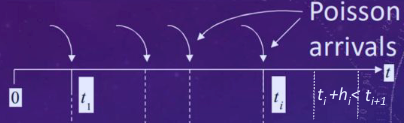
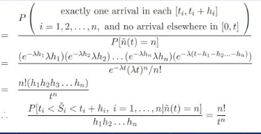
For $0 < s_1<s_2<\cdots<s_n\leq t$, the event $S_1 = s_1,S_2 = s_2,\cdots,S_n = s_n$ is equiva lent to the event that the first $n + 1$ inter - arrival times satisfy $T_1 = s_1,T_2 = s_2 - s_1,\cdots,T_n=s_n - s_{n - 1},T_{n+1}>t - s_n$.

Example #

Suppose that people immigrate into a territory at a Poisson rate $\lambda = 1$ per day.

1. What is the expected time until the tenth immigrant arrives?
2. What is the probability that the elapsed time between the tenth and the eleventh arrival exceeds two days? $$ (a)E[S_{10}]=\frac{10}{\lambda}=10\text{ days.} $$ $$ (b)P(t_{n}>2)=e^{-2\lambda}=e^{-2}\approx0.133. $$

Poisson Departures between Exponential Inter-arrivals #

Let $X(t)\sim P(\lambda t)$ and $Y(t)\sim P(\mu t)$ represent two independent Poisson processes called arrival and departure processes.

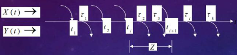
Let $Z$ represent the random interval between any two successive arrivals of $X(t)$. As discussed before, $Z$ has an exponential distribution with parameter $\lambda$.

Let $N$ represent the number of “departures” of $Y(t)$ between any two successive arrivals of $X(t)$.

Then from the Poisson nature of the departures we have $P{N = k|Z = t}=e^{-\mu t}\frac{(\mu t)^{k}}{k!}$.

Thus:

i.e., the random variable $N$ has a geometric distribution.

If arrivals and departures occur at a counter according to two independent Poisson processes, then the number of arrivals between any two departures has a geometric distribution. Similarly the number of departures between any two arrivals also represents another geometric distribution.

COMPOUND POISSON PROCESS #

A stochastic process ${X(t),t\geq0}$ is said to be a compound Poisson process if it can be represented as $X(t)=\sum_{i = 1}^{N(t)}Y_i$.

Here ${N(t),t\geq0}$ is a Poisson process, and ${Y_i,i\geq0}$ is a family of independent and identically distributed random variables that is also independent of $N(t)$.

Some examples:

1. If $Y_i\equiv1$, then $X(t)=N(t)$, and so we have the usual Poisson process.
2. Suppose that buses arrive at a sporting event in accordance with a Poisson process and suppose that the numbers of fans in each bus are assumed to be independent and identically distributed. Then ${X(t),t\geq0}$ is a compound Poisson process where $X(t)$ denotes the number of fans who have arrived by $t$, $Y_i$ represents the number of fans in the $i$ - th bus.
3. Suppose customers leave a supermarket in accordance with a Poisson process. If the $Y_i$, the amount spent by the $i$ - th customer, $i = 1,2,\cdots$, are iid, then ${X(t),t\geq0}$ is a compound Poisson process when $X(t)$ denotes the total amount of money spent by time $t$!

BULK ARRIVALS #

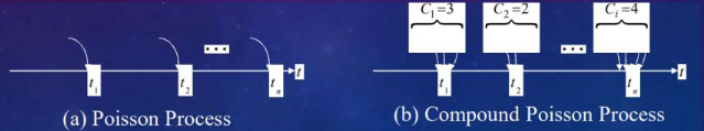
• Ordinary Poisson Process: One arrival at a time $(Y_i = 1)$
• Compound Poisson Process: At each arrival, $Y_i>1$ (more than one ➔BULK) arrivals at each $t_i$

COMPOUND POISON PROCESS #

Example: Suppose that families migrate to an area at a Poisson rate $\lambda = 2$ per week.

If the number of people in each family is independent and takes on the values $1,2,3,4$ with respective probabilities $1/6,1/3,1/3,1/6$, then what is the expected value and variance of the number of individuals migrating to this area during a fixed five-week period?

Letting $Y_i$ denote the number of people in the $i$-th family, we have

Hence, letting $X(5)$ denote the number of immigrants during a five - week period, then $E[X(5)] = 2\times5\times\frac{5}{2}=25$ and $Var[X(5)] = 2\times5\times\frac{43}{6}=\frac{215}{3}$

Related readings

• Random Walks
• Stochastic Processes
• Sequences of Random Variables
• Random Variables
• Repeated Trials