Random Variables
January 28, 2025 · 2 min read · Page View:
If you have any questions, feel free to comment below. Click the block can copy the code.
And if you think it's helpful to you, just click on the ads which can support this site. Thanks!
This article introduces the common distribution functions both continuous and discrete. Besides, the basic knowledge of conditional distribution such as total probability and Bayes’ Theorem is also introduced. The most important part are the Normal Approximation and Poisson Approximation of the Binomial Random Variable.
For the series of articles, you can find them in the Probability category.
Random variable X #
A random variable X is a process of assigning a number to every outcome, while the resulting function must stisfy the following two conditions (otherwise arbitrary):
- The set {X<=x) is an event for every x.
- The probabilities of the events(x= infinity) and (x=-infinity) equal 0.
Continuous, discrete, mixed
Prob. Distribution and their Properties #
Distribution Function #
The probability of the event $\({\xi | X(\xi) ≤x}\)$ must depend on x. Denote $\(P(\xi | X(\xi) ≤x)=F_{X}(x) ≥0 .\)$
- The role of X is to identify the actual r.v.
- $F_{X}(x)$ is said to the Probability Distribution Function of X.
eg. In the coin-tossing experiment, the probability of heads equals p and the probability of tails equals q. We define the random variable x such that X(h) =1, X(t)=0.
For the Distribution Function,
- If x < 0, because the X is 0 or 1, so it is impossible, so $F_{X}(x)=P(X\leq x)=0$.
- If $0\leq x < 1$, $F_{X}(x)=P(X\leq x)=P(X=0)=q$.
- If $x\geq 1$, $F_{X}(x)=P(X\leq x)=P(X=0 or X=1)=P(X=0)+P(X=1)=q+p=1$.

Properties #
A distribution function F(x) is nondecreasing, right-continuous and satisfies
- $P( \infty)=1$ and $P(-\infty)=0$
- if $x1 < x2$, then $F(x1) <= F(x2)$.
- $P(a<X<=b)=F(b)-F(a)$
- $P(X>a)=1-P(X<=a)=1-F(a)$
- $P(X=a)=F(a)-F(a-0)=F(a)-lim_{x->a-}F(x)$
Continuous, Discrete, (And Mixed) Types #
x is said to be a continuous type if its distribution function is continuous.
- Continuous: $F(x)$ is continuous and differentiable. $\[F_{X}(x-)=F_{X}(x) for all x ; P(X=x)=0.\]$
- Discrete: $F(x)$ is a step function. P(x=xi)=F(xi)-F(xi-0)=pi
- Mixed: $F(x)$ is a combination of continuous and discrete parts.
Prob. Density(PDF) #
- $f_{X}(x)=\frac{d F_{X}(x)}{d x}$
- $f_{X}(x)>=0$
- if $F_{X}(x)$ is continuous, then $f_{X}(x)$ will be a continuous function.
- if $X$ is a discrete type r.v, then its p.d.f has the general form $f_{X}(x)=\sum_{i} p_{i} \delta(x-x_{i})$ where $x_{i}$ represent the jump-discontinuity points in $F_{X}(x)$
- $F_{X}(x)=\int_{-\infty}^{x} f_{x}(u) d u .$
- $P{x_{1}<X(\xi) \leq x_{2}}=F_{X}\left(x_{2}\right)-F_{X}\left(x_{1}\right)=\int_{x_{1}}^{x_{2}} f_{X}(x) d x .$
Common Distribution Functions #
Parameter, shape, where to reach max, symmetrical…
Continuous Distribution #
Gaussian #

We say tbat x is a nonnal or Gaussian random variable if its density function is given by $f_{x}(x)=\frac{1}{\sqrt{2 \pi \sigma^{2}}} e^{-(x-\mu)^{2} / 2 \sigma^{2}}$ This is a bell-shaped curve, symmetric around the parameter μ ,and its distribution function is given by $F_{x}(x)=\int_{-\infty}^{x} \frac{1}{\sqrt{2 \pi \sigma^{2}}} e^{-(y-\mu)^{2} / 2 \sigma^{2}} d y \triangleq G\left(\frac{x-\mu}{\sigma}\right)$ where $G(x) \triangleq \int_{-\infty}^{x} \frac{1}{\sqrt{2 \pi}} e^{-y^{2} / 2} d y$
the notation x ~ $N(\mu, \sigma^{2})$ will be used to represent
Under very general conditions, the sum of a large number of independent random variables is approximately normally distributed.
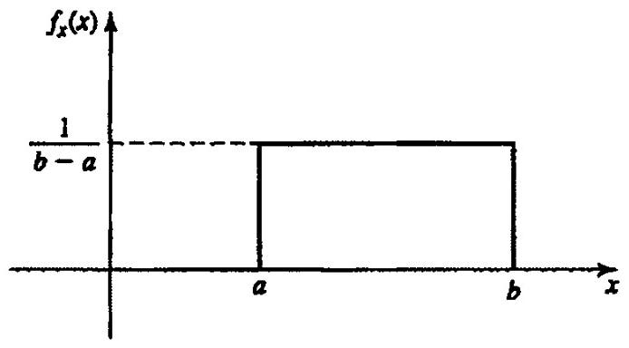
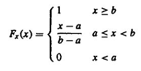
Uniform #


Exponential #

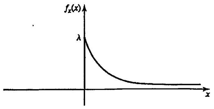
Exponential: X ~ $\varepsilon(\lambda)$
$$ f_{X}(x)=\begin{cases} \frac{1}{\lambda} e^{-\frac{x}{\lambda}}, & x \geq 0 \\ 0, & \text{otherwise} \end{cases} $$If the occurrences of events over non-overlapping intervals are independent (eg, arrival times of telephone calls/packets or bus arrival times at a bus stop, etc), then the waiting time distribution of these events can be modeled as exponential.
Memoryless property
$$P\{x>t+s | x>s\}=\frac{P\{x>t+s\}}{P\{x>s\}}=\frac{e^{-(t+s)}}{e^{-s}}=e^{-t}=P\{x>t\}$$eg. Suppose the life length of an appliance has an exponential distribution with \(\lambda=10\) years. A used appliance is bought by someone. What is the probability that it will not fail in the next 5 years?
$$P(x>t_{0}+5 | x>t_{0})=P(x>5)=e^{-5 / 10}=e^{-1 / 2}=0.368$$Discrete Distribution #
Bernoulli #
Bernoulli: X is Bernoulli distributed if X takes the values 1 and 0 with P{X = 1) = p, P{X = 0) = q = 1- P
Binomial #

With n independent Bernoulli trials, let Y be the total number of favorable outcomes.
$$ P(y=k)=\binom{n}{k} p^{k} q^{n-k} ,p+q=1, k=0,1,2, ..., n $$Poisson #
The number of occurrences of a rare event in a large number of trials. eg, the number of winning tickets among those purchased in a large lottery.
$$P(x=k)=e^{-\lambda} \frac{\lambda^{k}}{k !}, k=0,1,2, ...$$$$\frac{p_{k-1}}{p_{k}}=\frac{e^{-\lambda} \lambda^{k-1} /(k-1) !}{e^{-\lambda} \lambda^{k} / k !}=\frac{k}{\lambda}$$From the formula, the P(x=k) is the maximum when k=$\lambda$, if the $\lambda$ is an integer, the maximum is P(x=$\lambda$) and P(x=$\lambda$-1).
Geometric #
Mainly used to describe the first occurrence in the k-th trial in the series of independent trials.
$$X \sim g(p)$$$$P(X=k)=pq^k,k=0,1,2,..., q=1-p.$$Memoryless Property
$$P(x>m)=\sum_{k=m+1}^{\infty} P(x=k)=\sum_{k=m+1}^{\infty} p q^{k-1} =p q^{m}(1+q+\cdots)=\frac{p q^{m}}{1-q}=q^{m}$$$$P(x>m+n | x>m)=\frac{P(x>m+n)}{P(x>m)}=\frac{q^{m+n}}{q^{m}}=q^{n}$$Conclusion #
Common continuous probability distributions #
| Distribution | Description | Example |
|---|---|---|
| Normal distribution | Descrbes data with values that become less probable the farther they are from the mean, with a bell-shaped probability density function. | SAT scores |
| Continuous uniform | Describes data for which equal-sized intervais have equal probability. | The amount of time cars wait at a red light |
| Log-normal | Describes right-skewed data. It’s the probability distribution of a random variable whose logarthm is normaly distributed. | The average body weight of dfferent mammal species |
| Exponential | Describes data that has higher probablities for small values than large values.It’s the probablity distribution of time between independent events. | Time between earthquakes |
Common discrete probability distributions #
| Distribution | Description | Example |
|---|---|---|
| Bernoulli | Describes a single trial with two possible outcomes (e.g., success/failure, yes/no). | Tossing a coin |
| Binomial | Describes the number of successes in a fixed number of independent Bernoulli trials. | Number of heads in 10 coin tosses |
| Poisson | Describes the number of occurrences of an event in a fixed interval of time or space. | Number of phone calls received in an hour |
| Geometric | Describes the number of trials needed to get the first success in a sequence of independent Bernoulli trials. | Number of coin tosses until the first head |
Conditional Distributions #
$$P(A | B)=\frac{P(A \cap B)}{P(B)}, P(B) \neq 0 .$$The probaility distribution function $F_{X}(x)=P \lbrace X(\xi) ≤x \rbrace$ is a function of x.
Define the conditional distribution of the r.v X given the event B as
$$F_{X}(x | B)=P\lbrace X(\xi) \leq x | B\rbrace=\frac{P\lbrace (X(\xi) \leq x) \cap B\rbrace}{P(B)} .$$$$P\left(x_{1}Bayes’ Theorem in continuous version #

eg. 4-19 important.
Asymptotic Approximations for Binomial Random Variable #
Binomial Random Variable #
Let X represent a binomial random variable
$$P(k_{1} ≤X ≤k_{2})=\sum_{k=k_{1}}^{k_{2}} P_{n}(k)=\sum_{k=k_{1}}^{k_{2}}\binom{n}{k} p^{k} q^{n-k}$$And the coefficient $\binom{n}{k}$ grows rapidly as n increases.
The Normal Approximation (DeMoivre-Laplace Theorem) #
Suppose $\(n \to \infty\)$ with P held fixed. Then for k in the $\sqrt{n p q}$ neighborhood of $n p$, we can approximate
Important!
$$ \binom{n}{k} p^{k} q^{n-k} \simeq \frac{1}{\sqrt{2 \pi n p q}} e^{-(k-n p)^{2} / 2 n p q} ,p+q=1 $$Thus if $\(k_{1}\)$ and $\(k_{2}\)$ are within or around the neighborhood of the interval $\((n p-\sqrt{n p q}, n p+\sqrt{n p q}),\) we can approximate the summation by an integration
$$P(k_{1} ≤X ≤k_{2})=\int_{k_{1}}^{k_{2}} \frac{1}{\sqrt{2 \pi} \varphi p q} e^{-(x-u p)^{2} / 2 \varphi p q} d x=\int_{x_{1}}^{x_{2}} \frac{1}{\sqrt{2 \pi}} e^{-y^{2} / 2} d y,$$Important!
where $x_{1}=(k_{1}-n p) / \sqrt{n p q}$ and $x_{2}=(k_{2}-n p) / \sqrt{n p q}$
Define error function $\(erf(x)=\frac{1}{\sqrt{2 \pi}} \int_{0}^{x} e^{-y^{2} / 2} d y=erf(-x)\)$ that can be tabulated
$$P\left(k_{1} \leq X \leq k_{2}\right)=erf\left(x_{2}\right)-erf\left(x_{1}\right) .$$Meaning: the evaluation of the prob (k success in n trials) is approximately the evaluation of the normal curve.
Approximation of the P{k1<=X<=k2} #
When npq » 1 and k1 - np and k2 - np are of the order of $\sqrt{npq}$, the normal approximation is good.
$$ \sum_{k=k_{1}}^{k_{2}}\binom{n}{k} p^{k} q^{n-k} \simeq G\left(\frac{k_{2}-n p}{\sqrt{n p q}}\right)-G\left(\frac{k_{1}-n p}{\sqrt{n p q}}\right) $$Example 4-23 Over a period of 12 hours, 180 callsare made at random.What is the probability that in a four hour interval the number of calls is between 50 and 70?
Let p = 4/12, the probability that in a four hour interval the number of calls is between 50 and 70 is
The probability that k calls will occur in this interval equals
$$ \binom{180}{k}\left(\frac{1}{3}\right)^{k}\left(\frac{2}{3}\right)^{180-k} \simeq \frac{1}{4 \sqrt{5 \pi}} e^{-(k-60)^{2} / 80} $$and the probability that the number of calls is between 50 and 70 equals
$$ \sum_{k=50}^{70}\binom{180}{k}\left(\frac{1}{3}\right)^{k}\left(\frac{2}{3}\right)^{180-k} \simeq G(\sqrt{2.5})-G(-\sqrt{2.5}) \simeq 0.886 $$The Law of Large Numbers #
if an event A with P(A)=p, occurs k times in n trials, $k \approx np$ In fact
$$P(k=n p) \simeq \frac{1}{\sqrt{2 \pi n p q}} \to 0, n \to \infty$$the approximation $\(k \approx n p\)$ means that the ratio $\(k / n\)$ is close to p in the sense that, for any $\(\varepsilon>0\)$ the probability that $\(|k / n-p|<\varepsilon\)$ tends to 1 as $\(n \to \infty\)$
Possion Approximation #
For large n, the Gaussian approximation is valid only if p is fixed, i.e. if np » 1, npq » 1.
What if np is small, or if it does not increase with n?
p to 0 as n to infinity, so that np = $\(\lambda\)$ is fixed.
Recall as $\(n p=\lambda .\)$ We can obtain an excellent approximation:
$$ \begin{aligned} P_{n}(k) & =\frac{n(n-1) \cdots(n-k+1)}{n^{k}} \frac{(n p)^{k}}{k !}(1-n p / n)^{n-k} =\left(1-\frac{1}{n}\right)\left(1-\frac{2}{n}\right) \cdots\left(1-\frac{k-1}{n}\right) \frac{\lambda^{k}}{k !} \frac{(1-\lambda / n)^{n}}{(1-\lambda / n)^{k}} . \end{aligned} $$Thus The Poisson p.m.f
$$ lim_{n \to \infty, p \to 0, n p=\lambda} P_{n}(k)=\frac{\lambda^{k}}{k !} e^{-\lambda}, $$In conclusion:
If n to infinity, p to 0, and np = $\(\lambda\)$ is fixed, then
$$ \frac{n !}{k !(n-k) !} p^{k} q^{n-k} \underset{n \to \infty}{\to} e^{-\lambda} \frac{\lambda^{k}}{k !} k=0,1,2, ... $$eg. Example 4-27: A system contains 1000 components. Each component fails independently of the others and the probability of its failure in one month equals 10^-3. What the probability that in one month no failure occurs?
n = 1000, p = 10^-3, $\(\lambda\)$ = np = 1
$$ P_{1000}(X=0)=\frac{\lambda^{0}}{0 !} e^{-\lambda}=e^{-1} \simeq 0.368 $$eg. 4-8 The random variable x is $\(N(10 ; 1)\)$ .Find $\(f(x |(x-10)^{2}<4)\)$.
Random Poisson Points #
$$P\lbrace k in t_{a}\rbrace=\binom{n}{k} p^{k} q^{n-k} where, p=\frac{t_{a}}{T}$$Related readings
If you want to follow my updates, or have a coffee chat with me, feel free to connect with me: