Sequences of Random Variables
February 2, 2025 · 2 min read · Page View:
If you have any questions, feel free to comment below. Click the block can copy the code.
And if you think it's helpful to you, just click on the ads which can support this site. Thanks!
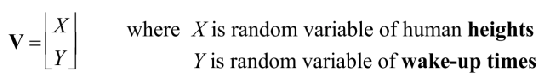
Random vector #
Substitute certain variables in $F(X.……,)y$ by $\infty$, we get the joint distribution of the remaining variables:
$F\left(x_{1}, x_{3}\right)=F\left(x_{1}, \infty, x_{3}, \infty\right)$
$f\left(x_{1}, x_{3}\right)=\int_{-\infty}^{\infty} \int_{-\infty}^{\infty} f\left(x_{1}, x_{2}, x_{3}, x_{4}\right) d x_{2} d x_{4}$
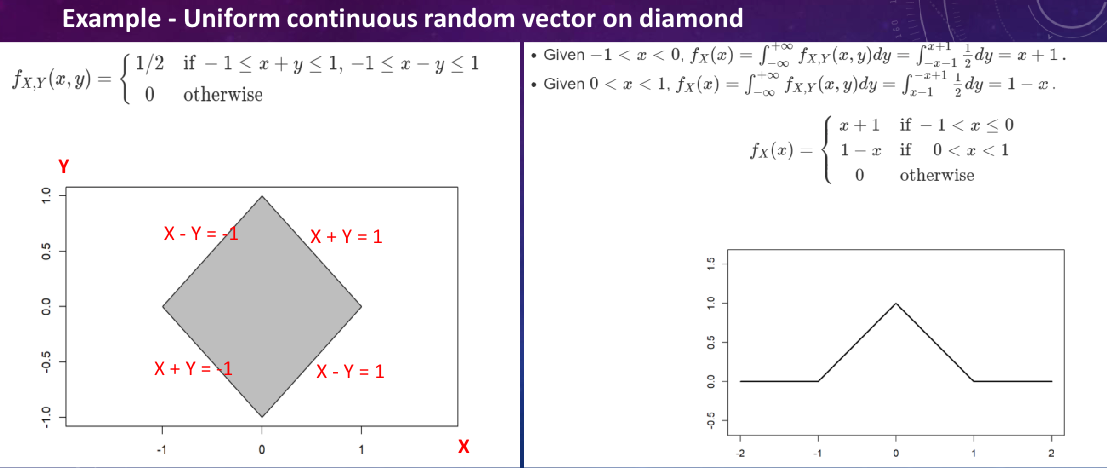
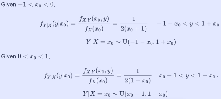
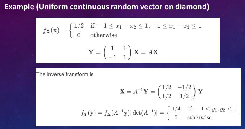
Example - Conditional dist. of uniform r.v. on diamond
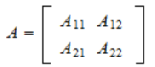
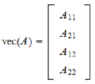
Random matrix #
Mean and Variance of Random Vector #
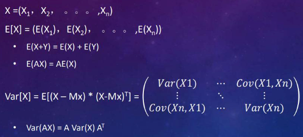
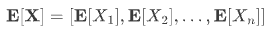
The Mx means the mean vector of X, which can be expressed as:
eg. 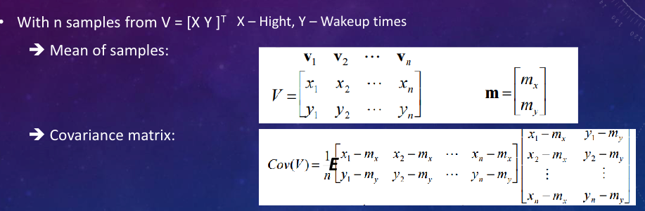
But if the two events are independent, then: Cov(X,Y) = 0 In the variance matrix there only will be Var(X) and Var(Y)
Functions of Random Vectors #
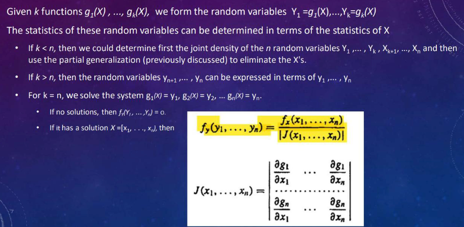
Density: Jacobin matrix #
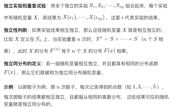
Independence & IID R.V.s #
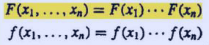
idd rvs
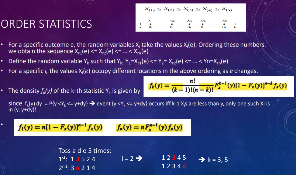
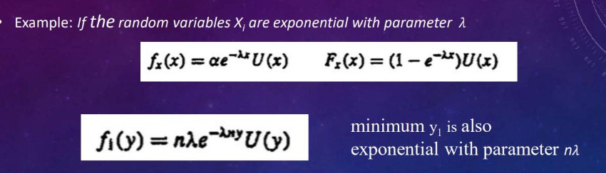
Order Statistics #
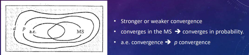
Stochastic convergence: different modes #
for a specific e, X(e) is a sequence of numbers that might or might not converge to a limit.
eg. X_n = n / (n + 1), n = 0, 1, 2, … The sequence converges to 1 when n to infinity.
which means in any neighborhood of 1,
∀ ε > 0, ∃ n_0(ε) s.t. for n ≥ n_0(ε) |X_n − 1| ≤ ε.
We can pick the $\epsilon$ to be very small, make sure the sequence will be trapped after reaching n_0(ε).
And as $\epsilon$ decreases, the n_0(ε) will increase. eg. when $\epsilon = 0.1$, n_0(ε) = 10; when $\epsilon = 0.01$, n_0(ε) = 100; when $\epsilon = 0.001$, n_0(ε) = 1001;

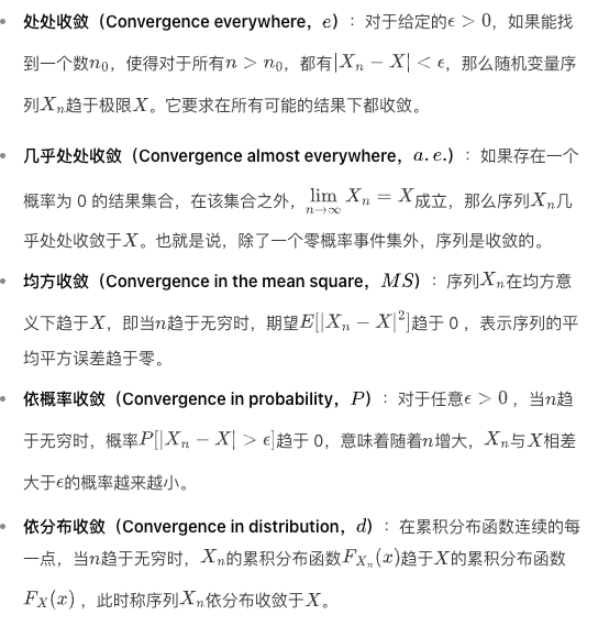
Convergence everywhere #
e. $X_n$ to $X$ as $n$ to $\infty$
a.e. $P(X_n$ to $X) = 1$ as $n$ to $\infty$
m.s. $E(|X_n - X|^2)$ to $0$ as $n$ to $\infty$
p. $P(|X_n - X| > \epsilon)$ to $0$ as $n$ to $\infty$
d. Fn(x) to F(x) as n to infinity
Limit Theorems #
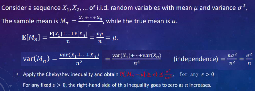
Let $S_{n}=X_{1}+\cdots+X_{n}$ be the sum of the first n measurements, the X1, X2.. of iid with mean $\mu$ and variance $\sigma^2$.
Because of independence,
$$ var\left(S_{n}\right)=var\left(X_{1}\right)+\cdots+var\left(X_{n}\right)=n \sigma^{2} $$With n increasing, the dist of S will spread out.
Direct research on $S_n$ cannot be done, but we can study the sample mean $M_n$.
$$ M_{n}=\frac{S_{n}}{n}=\frac{X_{1}+\cdots+X_{n}}{n} $$The law of large numbers #
As we disused before $E[M_{n}]=\mu_{n}$ var $(M_{n})=\frac{\sigma^{2}}{n}$
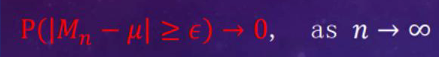
The variance of $M_n$ decreases to 0 as $n$ increases. And $M_n$ converges to $\mu$ as $n$ increases., which means the sample mean will converge to the real mean $\mu$.
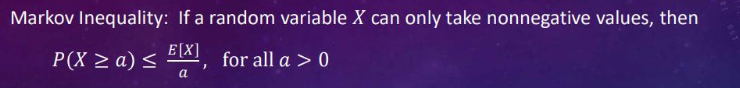
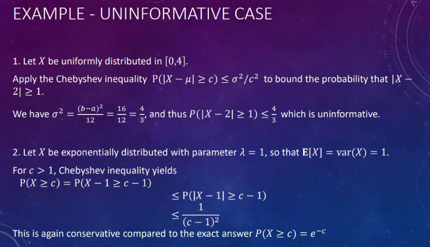
Markov and Chebyshev Inequalities #
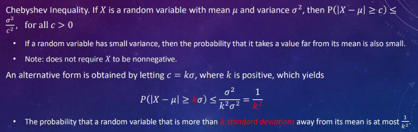
And if the sigma is unknown, for x in [a, b], we may use the bound (b-a)^2/4 as the substitute. for all c > 0.
Applications #
Weak Law of Large Numbers #
Central Limit Theorem #
The normaltive average defined as $Z_{n}=\frac{S_{n}-n \mu}{\sigma \sqrt{n}}$
- 1.subtract nu from \(S_{n}\) to obtain the zero-mean random variable \(S_{n}-n \mu\)
- 2.divide the result by $\sigma \sqrt{n}$ to get the normalized variable $Z_n$ Recall Var(Sn) = $n\sigma^2$
It can be seen that $E[Z_{n}]=0$ var $\([Z_{n}] = 1\)$
So when n increases to infinity, the distribution of $Z_n$ will be close to the standard normal distribution.
So the mean or var will independent of n.
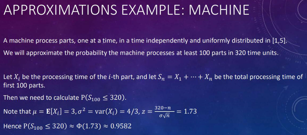
The approximations based on ctl #
Let $S_{n}=X_{1}+\cdots+X_{n}$ where the X are iid.random variables with mean u, variance $\sigma^2$
If n is large, the probability \(P(S_{n} ≤c)\) can be approximated by treating \(S_{n}\) as if it were normal, according to the following procedure. Pay attention to the c!!!
- calculate the mean $n\mu$ and variance $n\sigma^2$
- calculate the normalized variable $Z_n = \frac{S_n - n\mu}{\sigma\sqrt{n}}$
- use the approximation $\(P(S_{n} ≤c) ≈\Phi(z)\)$
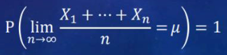
Strong Law of Large Numbers #
Related readings
If you want to follow my updates, or have a coffee chat with me, feel free to connect with me: