Stochastic Processes

March 15, 2025 · 20 min read · Page View:

If you have any questions, feel free to comment below.

Compared to deterministic model, which is specified by a set of equations that describe exactly how the system will evolve over time. In a stochastic model, the evolution is at least partially random and if the process is run several times, it will not give identical results.

Introduction #

Stochastic Processes #

Let $\xi$ be the random result of an experiment, and for each such result, there is a waveform $X(t,\xi)$. Here, $t$ usually represents time, and $\xi$ represents a random factor.

• The set of these waveforms constitutes a stochastic process.
• The random result set ${\xi_k}$ and the time index $t$ can be continuous or discrete(countable infinite or finite).

eg. Brownian motion, stock market, queue system.

Compare with RV #

• R.V. X: A rule that assigns a number $x(e)$ to every outcome $e$ of an experiment $S$.
• Random/stochastic process $X(t)$: A family of time functions depending on the parameter $e$, or equivalently, a function of both $t$ and $e$. Here, $S={e}$ represents all possible outcomes, and $R = {\text{possible values for }t}$.
• Continuous vs Discrete:
  • If $R$ is the real axis, $X(t)$ is a continuous - state process.
  • If $R$ takes only integer values, $X(t)$ is a discrete - state process, also known as a random sequence ${X_n}$ with countable values.

Interpretations of $X(t)$ #

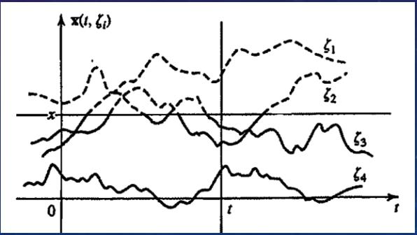
1. When $t$ and $e$ are variables, it is a family of functions $x(t,e)$.
2. When $t$ is a variable and $e$ is fixed, it is a single time function (or a sample of the given process).
3. When $t$ is fixed and $e$ is variable, $x(t)$ is a random variable representing the state of the given process at time $t$.
4. When $t$ and $e$ are fixed, $x(t)$ is a number.

Continuous vs Discrete #

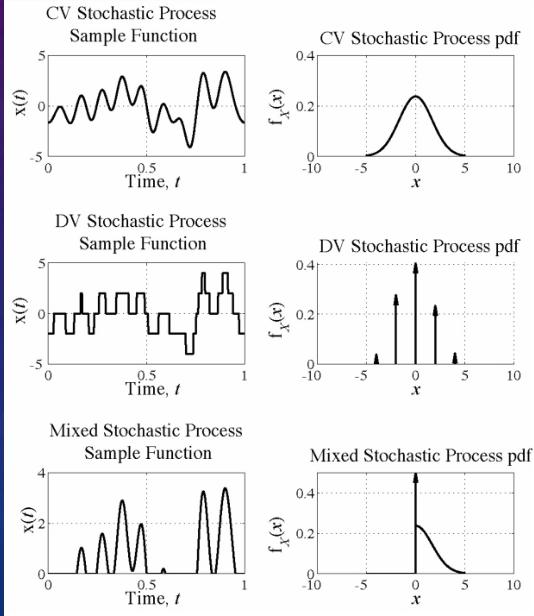
DTCV Process - Record the temperature #

This is a discrete time, continuous value (DTCV) stochastic process. eg. Record the temperature at noon every day for a year.

DTDV Process - People flipping coins #

This is a discrete time, discrete value (DTDV) stochastic process. eg. Suppose there is a large number of people, each flipping a fair coin every minute. Assigning the value 1 to a head and 0 to a tail.

CTCV Process – Brownian Motion #

The motion of microscopic particles colliding with fluid.

• Molecules results in a process $X(t)$ that consists of the motions of all particles.
• A single realization $X(t,\xi_i)$ is the motion of a specific particle (sample).

Regular Process #

Under certain conditions, the statistics of a regular process $X(t)$ can be determined from a single sample.

Predictable Process – Voltage of AC Generator #

For $x(t)=r\cos(\omega t + \varphi)$ where both the amplitude $r$ and phase $\varphi$ are random, a single sample is $x(t,\xi_i)=r(\xi_i)\cos[\omega t+\varphi(\xi_i)]$. This process is a family of pure sine waves and is completely specified and predictable (or deterministic) with random variables $r$ and $\varphi$.

However, a single sample does not fully specify the properties of the entire process as it depends on the specific values of $r(\xi)$ and $\varphi(\xi)$.

Equality #

Two stochastic processes $X(t)$ and $Y(t)$ are equal (everywhere) if their respective samples $X(t)$ and $Y(t)$ are equal in the mean-square (MS) sense, i.e., $E{|X(t)-Y(t)|^{2}}=0$, or $X(t,\xi)=Y(t,\xi)$ for all sample $\xi$(X(t, $\xi$) - Y(t, $\xi$) = 0 with probability 1 -> w.p.1).

First-Order Distribution & Density Function #

If $X(t)$ is a stochastic process, for a fixed $t$, $X(t)$ represents a random variable.

Its distribution function is $F_{x}(x,t)=P{X(t)\leq x}$, which depends on $t$ since different $t$ values result in different random variables, means fixed $t$, $X(t)$ will not exceed $x$ with probability $F_{x}(x,t)$.

The first-order probability density function of the process $X(t)$ is $f_{x}(x,t)=\frac{dF_{x}(x,t)}{dx}$.

Frequency Interpretation #

For $X(t,\xi)$, if we conduct $n$ experiments with outcomes $\xi_i$ ($i = 1,\cdots,n$), we get $n$ functions $X(t,\xi_i)$.

Let $n_{t}(x)$ be the number of trials such that at time $t$, $x(t,\xi)\leq x$. Then $F(x,t)\approx\frac{n_{t}(x)}{n}$. So we can think of $F(x,t)$ as the probability that $X(t)$ will not exceed $x$, when the n is large.

Second-Order and N-th Order Properties #

• Second - Order Distribution/Density Function: For $t = t_1$ and $t = t_2$, $X(t)$ represents two different random variables $x_1 = X(t_1)$ and $x_2 = X(t_2)$. Their joint distribution is $F_{x}(x_1,x_2,t_1,t_2)=P{X(t_1)\leq x_1,X(t_2)\leq x_2}$, and the joint density function is $f_{x}(x_1,x_2,t_1,t_2)=\frac{\partial^{2}F_{x}(x_1,x_2,t_1,t_2)}{\partial x_1\partial x_2}$. Given $F(x_1,x_2,t_1,t_2)$, we can find $F(x_1,t_1)=F(x_1,\infty,t_1,t_2)$ and $f(x_1,t_1)=\int_{-\infty}^{\infty}f(x_1,x_2,t_1,t_2)dx_2$.
• N-th Order Density Function: $f_{x}(x_1,x_2,\cdots,x_n,t_1,t_2,\cdots,t_n)$ represents the $n$-th order density function of the process $X(t)$. Completely specifying the stochastic process $X(t)$ requires knowing $f_{x}(x_1,x_2,\cdots,x_n,t_1,t_2,\cdots,t_n)$ for all $t_i$ ($i = 1,2,\cdots,n$) and all $n$, which is almost impossible in reality.

Second-Order Properties #

* means Complex Conjugate

• Mean Value: The mean value of a process $X(t)$ is: $$ \mu(t)=E\{X(t)\}=\int_{-\infty}^{+\infty}xf_{x}(x,t)dx $$

In general, the mean of a process can depend on the time index $t$.

• Autocorrelation Function: Defined as $$ R_{xx}(t_1,t_2)=E\{X(t_1)X^{\ast}(t_2)\}=\iint x_1 x_1^{\ast}f_{x}(x_1,x_2,t_1,t_2)dx_1dx_2 $$
  • It satisfies $R_{xx}(t_1,t_2)=R_{xx}^{*}(t_2,t_1)$ and is a non-negative definite function.
  • i.e., $\sum_{i = 1}^{n}\sum_{j = 1}^{n}a_{i}a_{j}^{*}R_{xx}(t_i,t_j)\geq0$ for any set of constants ${a_{i}}_{i = 1}^{n}$.
  • The average power of $X(t)$ is $E{|X(t)|^{2}}=R_{xx}(t,t)>0$.
• Autocovariance: The autocovariance of the random variables $X(t_1)$ and $X(t_2)$ is $C_{xx}(t_1,t_2)=R_{xx}(t_1,t_2)-\mu_{x}(t_1)\mu_{x}^{*}(t_2)$.
  • $C_{xx}(t, t) = Var(X(t))$

Examples #

1. For a deterministic $x(t)$, specific calculations can be made according to relevant rules.
2. Given a process with $\mu(t)=3$ and $R(t_1,t_2)=9 + 4e^{-0.2|t_2 - t_1|}$, we can calculate the means, variances, and covariances of related random variables.
3. For $z=\int_{-T}^{T}X(t)dt$, $E[|z|^{2}]=\int_{-T}^{T}\int_{-T}^{T}E{X(t_1)X^{*}(t_2)}dt_1dt_2=\int_{-T}^{T}\int_{-T}^{T}R_{xx}(t_1,t_2)dt_1dt_2$.
4. For $X(t)=a\cos(\omega_0t+\varphi)$ with $\varphi\sim U(0,2\pi)$, $\mu_{x}(t)=0$ and $R_{xx}(t_1,t_2)=\frac{a^{2}}{2}\cos\omega_0(t_1 - t_2)$.

Possion Random Variable #

For the $t$ ，$X(t)$ is a Poisson random variable with parameter $\lambda t$ ，its mean $E{X(t)}=\eta(t)=\lambda t$ 。This indicates that the average level of the value of the random variable at time $t$ is determined by $\lambda t$ , and $\lambda$ can be understood as the average rate of events occurring in a unit time.

• Autocorrelation Function: $$ R(t_1,t_2)=\begin{cases}\lambda t_2+\lambda^{2}t_1t_2 & t_1\geq t_2\\\lambda t_1+\lambda^{2}t_1t_2 & t_1\leq t_2\end{cases} $$ it describes the correlation degree between the Poisson process at different times $t_1$ and $t_2$ 。
• Autocovariance Function： $$ C(t_1,t_2)=\lambda\min(t_1,t_2)=\lambda t_1U(t_2 - t_1)+ \lambda t_2U(t_1 - t_2) $$ where $U(\cdot)$ is the unit step function. The autocovariance measures the degree of deviation of random variables from their respective means at different times.

Properties of Independent Poisson Processes #

• Sum of Independent Poisson Processes: If $X_1(t)$ and $X_2(t)$ are independent Poisson processes with parameters $\lambda_1t$ and $\lambda_2t$ respectively, then their sum $X_1(t)+X_2(t)$ is also a Poisson process with parameter $(\lambda_1 + \lambda_2)t$. This property highlights the special nature of Poisson processes when dealing with multiple independent, similar random event streams.
• Difference of Independent Poisson Processes: The difference $X_1(t)-X_2(t)$ of two independent Poisson processes is not a Poisson process, indicating that Poisson processes do not possess the simple properties of addition and subtraction like other random processes.

Point and Renewal Processes #

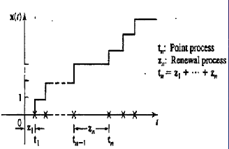
• Point Process: A set of random points $t$ on the time axis. Defining a stochastic process $X(t)$ as the number of points in the interval $(0,t)$ gives a Poisson process.
• Renewal Process: For a point process, we can associate a sequence of random variables $Z_1 = t_0$, $Z_n=t_n - t_{n - 1}$. This sequence is called a renewal process.
• This can be exemplified by the life history of light bulbs(renewal processes $Z_n$) that are replaced when they fail(point processes $t_n$).

Poisson Process #

• Properties:
  • P1: The number $n(t_1,t_2)$ of points $T_i$ in an interval $(t_1,t_2)$ of length $t=t_2 - t_1$ is a Poisson random variable with parameter $\lambda t$, i.e., $$ P\{n(t_1,t_2)=k\}=\frac{e^{-\lambda t}(\lambda t)^{k}}{k!} $$
  • P2: If the intervals $(t_1,t_2)$ and $(t_3,t_4)$ are non-overlapping, then the random variables $n(t_1,t_2)$ and $n(t_3,t_4)$ are independent.
• Defining $X(t)=n(0,t)$ gives a discrete-state process consisting of a family of increasing staircase functions with discontinuities at the points $t_i$.

Random Selection of Poisson Points #

Let $X(t)\sim P(\lambda t)$ be a Poisson process with parameter $\lambda t$. If each occurrence of $X(t)$ is tagged (selected) independently with probability $p$, then $Y(t)$ (the total number of tagged events in $(0,t)$) $\sim P(\lambda p t)$ and $Z(t)$ (the total number of un-tagged events in $(0,t)$) $\sim P(\lambda q t)$ ($q = 1 - p$).

Poisson Points and Binomial Distribution #

For $t_1\lt t_2$,

for $k = 0,1,\cdots,n$.

Given that only one Poisson occurrence has taken place in an interval of length $T$, the conditional probability density function of the corresponding arrival instant is uniform in that interval.

Some General Properties #

• The statistical properties of a real stochastic process $x(t)$ are completely determined by its $n$-th order distribution. $F_x(x_1,x_2,\cdots,x_n,t_1,t_2,\cdots,t_n)$.
• Autocorrelation: $R_{xx}(t_1,t_2)=E\{x(t_1)x^{\ast}(t_2)\}$ is a positive-definite function, $R(t_2,t_1)=E\{x(t_2)x^{\ast}(t_1)\}=R^{*}(t_1,t_2)$ and $R(t,t)=E{|x(t)|^{2}}\geq0$.
• Autocovariance: $C(t_1,t_2)=R(t_1,t_2)-\eta(t_1)\eta^{*}(t_2)$ with $\eta(t)=E{x(t)}$.
• Correlation Coefficient: $r(t_1,t_2)=\frac{C(t_1,t_2)}{\sqrt{C(t_1,t_1)C(t_2,t_2)}}$.
• Cross-Correlation: The cross-correlation of two processes $X(t)$ and $Y(t)$ is $R_{xy}(t_1,t_2)=E\{x(t_1)y^{\ast}(t_2)\}=R_{yx}^{*}(t_2,t_1)$.
• Cross-Covariance: Their cross-covariance is $C_{x,y}(t_1,t_2)=R_{xy}(t_1,t_2)-\eta_{x}(t_1)\eta_{y}^{*}(t_2)$.

Relationships Between Two Processes #

• Orthogonal: Two processes $X(t)$ and $Y(t)$ are (mutually) orthogonal if $R(t_1,t_2)=0$ for every $t_1$ and $t_2$.
• Uncorrelated: They are uncorrelated if $C(t_1,t_2)=0$ for every $t_1$ and $t_2$. This means that the two processes are independent at different times.
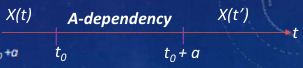
• $\alpha$-dependent Processes: If values $x(t)$ for $t\lt t_0$ and $t\gt t_0+\alpha$ are mutually independent, then $C(t_1,t_2)=0$ for $|t_1 - t_2|>\alpha$.

• Independent: The two processes are independent if $X(t_1)$…$X(t_n)$ and $Y(t_1)$…$Y(t_n)$ are mutually independent.
• White Noise: A process $V(t)$ is white noise if its values $V(t_i)$ and $V(t_j)$ are uncorrelated for every $t_i\neq t_j$ ($C(t_i,t_j)=0$). If $V(t_i)$ and $V(t_j)$ are not only uncorrelated but also independent, then $V(t)$ is strictly white noise and $E[V(t)] = 0$.

Normal Processes #

For any $n$ and any time $t_1$,⋯,$t_n$, the random variables $X(t_1)$…$X(t_n)$ are jointly normal.

• The first-order density function $f(x,t)$ is the normal density $N[\eta(t);\sqrt{C(t,t)}]$, which means that only the mean and autocovariance at a specific time are needed to determine the probability density function of the random variable at that time.
• The second-order density function $f(x_1,x_2;t_1,t_2)$ is the joint normal density $N(\eta_1(t),\eta_2(t);\sqrt{C(t_1,t_1)},\sqrt{C(t_2,t_2)},r(t_1,t_2))$, which involves the means, autocovariances, and correlation coefficients of two different times, representing the joint probability distribution of the random variables at these two times.
• Given any function $\eta(t)$ and a positive-definite function $C(t_1,t_2)$, we can construct a normal process with mean $\eta(t)$ and autocovariance $C(t_1,t_2)$. This indicates that theoretically, we can construct a normal random process according to specific mean function and autocovariance function.

Stationary Stochastic Processes #

Stationary processes exhibit statistical properties that are invariant to shift in the time index.

Strict-Sense Stationarity #

• First-order stationarity: The processes $X(t)$ and $X(t + c)$ have the same statistics for any $c$.
• Second-order stationarity: The processes ${x(t_1),x(t_2)}$ and ${X(t + c),X(t_2 + c)}$ have the same statistics for any $c$.
• A process is nth-order strict-sense stationary if $f_{x}(x_1,x_2,\cdots,x_n,t_1,t_2,\cdots,t_n)\equiv f_{x}(x_1,x_2,\cdots,x_n,t_1 + c,t_2 + c,\cdots,t_n + c)$ for any $c$, all $i = 1,\cdots,n$, and $n = 1,2,\cdots$.

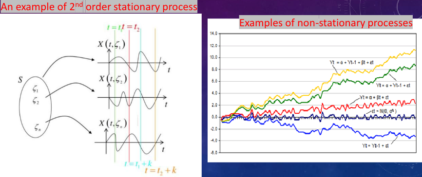
• For a first-order strict-sense stationary process, $f_{x}(x,t)\equiv f_{x}(x,t + c)$ for any $c$, and $E[X(t)] = \int_{-\infty}^{\infty}xf_{x}(x)dx = \mu$ is a constant.
• For a second-order strict-sense stationary process, the second-order density function depends only on the difference of the time indices $t_1 - t_2 = \tau$, and the autocorrelation function $R_{xx}(t_1,t_2)=R_{xx}(t_1 - t_2)$.

In that case the autocorrelation function is given by

Wide-Sense Stationarity #

A process $X(t)$ is wide-sense stationary if:

1. $E\{X(t)\}=\mu$ (constant)
2. Autocorrelation function: $E\{X(t_1)X^{*}(t_2)\}=R_{xx}(t_1 - t_2)$

Strict-sense stationarity always implies wide-sense stationarity, but the converse is generally not true, except for Gaussian processes. For a Gaussian process, wide-sense stationarity implies strict-sense stationarity because the joint probability density function of Gaussian random variables depends only on their second-order statistics. The Gaussian process:

In general, in the Gaussion Process, the wide sense stationary process(w.s.s) $\Rightarrow$ strict-sense stationary(s.s.s).

• Examples:
  • For a white noise process, $E{V(t)}=0$ and $E{V(t_1)V^{*}(t_2)}=0$ for $t_1\neq t_2$.
  • For a Poisson process, $E{n(t)}=\lambda t$ and $E{n(t_1)n(t_2)}=\lambda^2t_1t_2$ for $t_1\neq t_2$.

Centered Process #

• Given a process $X(t)$ with mean $\eta(t)$ and autocovariance $C_{x}(t_1,t_2)$. The difference $\bar{X}(t)=X(t)-\eta(t)$ is called the centered process associated with the $X(t)$.
• $E{\bar{X}(t)} = 0$, $R_{\bar{X}}(t_1,t_2)=C_{x}(t_1,t_2)$.
  • Due to the fact that $E{\bar{X}(t)} = 0$(which meets the requirement that the mean is constant), and if the process $X(t)$ is covariance stationary, that is, if $C_{x}(t_1,t_2)=C_{x}(t_1 - t_2)$ = $C_{x}(t_2 - t_1)$ = $R_{\bar{X}}(t_1,t_2)$, then its centered process $\bar{X}(t)$ is WSS.

OTHER FORMS OF STATIONARITY #

• Asymptotically stationary: if the statistics of the r.v. $X(t_1 + c), \ldots, X(t_n + c)$ do not depend on $c$ if $c$ is large. More precisely, the function $f(x_1,\ldots,x_n, t_1 + c, \ldots, t_n + c)$ tends to a limit (that does not depend on $c$) as $c \to \infty$.

• Nth-order stationary: if $f_x(x_1,x_2,\cdots,x_n, t_1,t_2,\cdots,t_n) \equiv f_x(x_1,x_2,\cdots,x_n, t_1 + c,t_2 + c,\cdots,t_n + c)$ holds not for every $n$, but only for $n <= N$

• Stationary in an interval: if the above holds for every $t_i$ and $t_i + c$ in this interval.

• $X(t)$ is a process with stationary increments if its increments $Y(t)=X(t + h)-X(t)$ form a stationary process for every $h$. Remember the Poisson process?

MEAN SQUARE PERIODICITY #

• MS periodic if $E{|X(t + T)-X(t)|^2}=0$ for every $t$
  • For a specific $t$, $X(t + T)=X(t)$ w.p. 1 with probability 1
• A process $X(t)$ is MS periodic iff(if and only if) its autocorrelation is doubly periodic, that is, if $R(t_1 + mT, t_2 + nT)=R(t_1, t_2)$ for every integer $n$ and $m$.

STOCHASTIC SYSTEMS #

A few components of stochastic systems:

• Random time-delays
• Noisy (modelled as random) disturbances
• Stochastic dynamic processes

STOCHASTIC MODELS #

The resulting distribution provides an estimate of which outcomes are most likely to occur and the potential range of outcomes.

Creating a stochastic model involves a set of “equations” with inputs that represent uncertainties over time. Therefore, stochastic models will produce different results every time the model is run.

HOW STOCHASTIC MODELS WORK? #

To estimate the probability of each outcome, one or more of the inputs must allow for random variation over time. It results in an estimation of the probability distributions.

Systems with Stochastic Inputs #

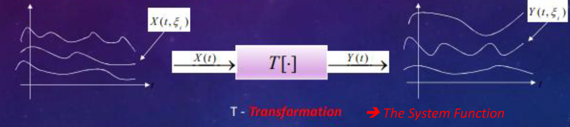
A deterministic system transforms each input waveform $X(t, \xi_{i})$ into an output waveform $Y(t, \xi_{i}) = T[X(t, \xi_{i})]$ operating only on the time variable $t$. Thus a set of realizations at the input corresponding to a process $X(t)$ generates a new set of realizations $Y(t,\xi_{i})$ at the output associated with a new process $Y(t)$.

Our goal is to study the output process statistics in terms of the input process statistics and the system function.

A stochastic system on the other hand operates on both the variables $t$ and $\xi$.

• RANDOM BINARY SEQUENCE: $\zeta=\sum_{i=1}^{\infty} b_{i} 2^{-i}, b_{i} \in{0,1} .$ $P[X(1, \zeta)=0]=P\left[0\leq\zeta<\frac{1}{2}\right]=\frac{1}{2}$ $P[X(1, \zeta)=0\text{ and }X(2, \zeta)=1]=P\left[\frac{1}{4}\leq\zeta<\frac{1}{2}\right]=\frac{1}{4}$ since all points in the interval $[0\leq\zeta\leq1]$ begin with $b_{1}=0$ and all points in $[\frac{1}{4},\frac{1}{2})$ begin with $b_{1}=0$ and $b_{2}=1$. Clearly, any sequence of $k$ bits has a corresponding subinterval of length (and hence probability) $2^{-k}$.

• RANDOM SINUSOIDS

  • $X(t, \zeta)=\zeta\cos(2\pi t),-\infty<t<\infty$
  • $Y(t, \zeta)=\cos(2\pi t+\zeta),-\infty<t<\infty$

• BINOMIAL COUNTING PROCESS

  • Let $X_{n}$ be a sequence of independent, identically distributed Bernoulli random variables with $p = 1/2$.
  • Let $S_{n}$ be the number of 1 in the first $n$ trials: $S_{n}=X_{1}+X_{2}+\cdots+X_{n}\text{ for }n = 0,1,…$
  • $S_{n}$ is a binomial random variable with parameters $n$ and $p = 1/2$.

• FILTERED NOISY SIGNAL(Additive Noise)

  • Let $x_{j}$ be a sequence of independent, identically distributed observations of a signal voltage $\mu$ corrupted by zero-mean Gaussian noise $N_{j}$ with variance $\sigma^{2}$: $X_{j}=\mu+N_{j}\text{ for }j = 0,1,…$
  • Consider the signal that results from averaging the sequence of observations: $S_{n}=\left(X_{1}+X_{2}+\cdots+X_{n}\right)/n\text{ for }n = 0,1,…$
  • From previous chapters we know that $S_{n}$ is the sample mean of an i.i.d sequence of Gaussian random variables. We know that $S_{n}$ itself is a Gaussian random variable with mean $\mu$ and variance $\sigma^{2}/n$, and so it tends towards the value $\mu$ as $n$ increases.

K-TH ORDER JOINT CUMULATIVE DISTRIBUTION FUNCTION #

Let $X_{1},X_{2},…,X_{n}$ be the $k$ random variables obtained by sampling the random process $X(t, \zeta)$ at the times $t_{1},t_{2},\ldots,t_{k}$, $X_{1}=X\left(t_{1}, \zeta\right),X_{2}=X\left(t_{2}, \zeta\right),…,X_{k}=X\left(t_{k}, \zeta\right)$

Then

Discrete Case:

DETERMINISTIC VS. STOCHASTIC #

Transformation $T: Y(t)=T[X(t)]$ is:

• deterministic if it operates only on the variable $t$ treating $\xi$ as a parameter.
• stochastic if $T$ operates on both variables $t$ and $\xi$. There exist two outcomes $\xi_{1}$ and $\xi_{2}$ such that $X(t, \xi_{1}) = X(t, \xi_{2})$ identically in $t$ but $Y(t, \xi_{1})\neq Y(t, \xi_{2})$.

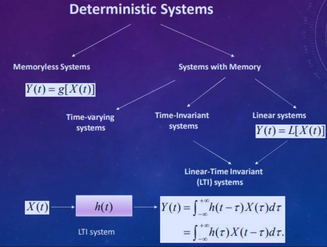
Memoryless Systems #

• Memoryless: $Y(t)=2X(t)$, and $Y(t)=\cos(X(t))$
• Not-memoryless: $Y(t)=X(t + \tau)+X(t)$, and $Y(t)=X(t)e^{X(t-\tau)}$

The output $Y(t)$ in this system depends only on the present value of the input $X(t)$, $Y(t)=g{X(t)}$. The current output value $Y(t)$ can be determined from knowing only the value of the current input $X(t)$.

• Strict-sense stationary input -> Memoryless system -> Strict-sense stationary output.
• Wide-sense stationary input -> Memoryless system -> Need not be stationary in any sense.
• $x(t)$ stationary Gaussian with Memoryless system, $Y(t)$ stationary, but not Gaussian with $R_{Y}(\tau)=\eta^2R_{X}(\tau)$.

STATISTICS OF Y = G[X(T)] #

• 1st order: $f_{y}(y ; t)\to f_{x}(x ; t)$, similar as for functions of random variables $E{y(t)}=\int_{-\infty}^{\infty}g(x)f_{x}(x ; t)dx$

• 2nd order: $f_{y}(y_{1},y_{2} ; t_{1},t_{2})\to f_{x}(x_{1},x_{2} ; t_{1},t_{2})$

  $$ E\left\{y\left(t_{1}\right)y\left(t_{2}\right)\right\}=\int_{-\infty}^{\infty}\int_{-\infty}^{\infty}g\left(x_{1}\right)g\left(x_{2}\right)f_{x}\left(x_{1},x_{2} ; t_{1},t_{2}\right)dx_{1}dx_{2} $$

• nth - order: $f_{y}(y_{1},…,y_{n} ; t_{1},…,t_{n})\to f_{x}(x_{1},…,x_{n} ; t_{1},…,t_{n})$ need to solve the system $g(x_{1}) = y_{1},\cdots,g(x_{n}) = y_{n}$. If this system has a unique solution $f_{y}\left(y_{1},…,y_{n} ; t_{1},…,t_{n}\right)=\frac{f_{x}\left(x_{1},…,x_{n} ; t_{1},…,t_{n}\right)}{\left|g^{\prime}\left(x_{1}\right)\cdots g^{\prime}\left(x_{n}\right)\right|}$

• If $X(t)$ is stationary of order N, then $Y(t)$ is stationary of order $N$.

• If $X(t)$ is stationary in an interval, then $Y(t)$ is stationary in the same interval.

• If $x(t)$ is WSS stationary, then $y(t)$ might not be stationary in any sense.

SQUARE - LAW DETECTOR #

A memory-less system whose output equals $Y(t)=X^{2}(t)$. The system $y = x^{2}$ has the two solutions $\pm\sqrt{y}$ and $y^{\prime}(x)=\pm2\sqrt{y}$

If $y_{1}>0$ and $y_{2}>0$, then the system $y_{1}=x^{2},y_{2}=x^{2}$ has the four solutions $(\pm\sqrt{y_{1}},\pm\sqrt{y_{2}})$. Its Jacobian is $\pm4\sqrt{y_{1}y_{2}}$

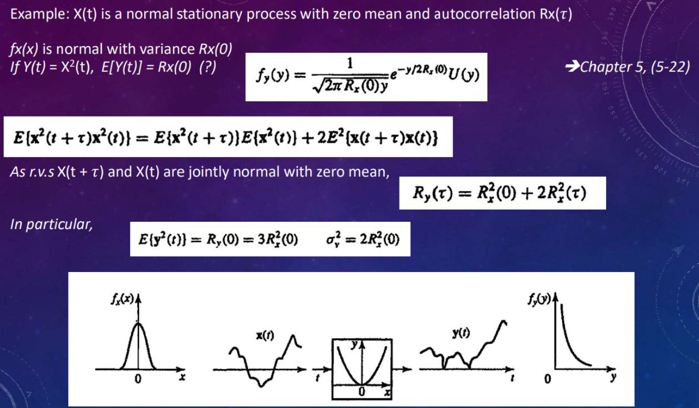
HARD LIMITER #

A memoryless system with $g(x)=\begin{cases}1& \text{if }x>0\ - 1& \text{else}\end{cases}$

Linear Systems #

$L$ represents a linear system if for any $a_{1},a_{2},X_{1}(t),X_{2}(t)$:

True even if $a_{1},a_{2}$ are r.v.s.

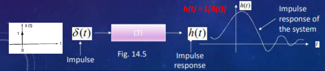
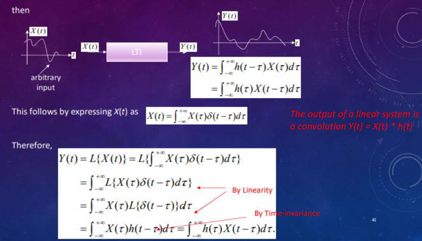
Let $Y(t)=L\{X(t)\}$ represent the output of a linear system.

Time Invariant System #

$L$ represents a time invariant system if $Y(t)=L{X(t)}\Rightarrow L\{X(t - t_{0})\}=Y(t - t_{0})$. Shift in the input results in the same shift in the output also.

• If $L$ satisfies both equations, then it corresponds to a linear time invariant (LTI) system.
• LTI systems can be uniquely represented in terms of their output to a delta function $h(t)=L[\delta(t)]$, the system impulse response. Then $Y(t)=\int_{-\infty}^{+\infty}h(t-\tau)X(\tau)d\tau=\int_{-\infty}^{+\infty}h(\tau)X(t-\tau)d\tau$

FUNDAMENTAL THEOREM #

• For any linear system $E\{L[X(t)]\}=L[E\{X(t)\}]$
  • $\eta_y(t)=L[\eta_x(t)]$
  • $E{y(t)}=\int_{-\infty}^{\infty}E\{x(t - \alpha)\}h(\alpha)d\alpha=\eta_x(t)*h(t)$
• Frequency interpretation: At the $i$-th trial the input to the system is a function $X(t,\xi_i)$ yielding output function $Y(t,\xi_j)=L[X(t,\xi_j)]$.

For large $n$,

Output Statistics #

The mean of the output process:

The cross-correlation function between the input and output processes is:

Finally the output autocorrelation function is given by:

or

Review that:

So in finally, we can deduce that:

In particular if $X(t)$ is wide-sense stationary

• We have $\mu_x(t)=\mu_x$

  $$ \mu_y(t)=\mu_x\int_{-\infty}^{\infty}h(\tau)d\tau=\mu_x c, \text{ a constant} $$

• Also $R_{xx}(t_1,t_2)=R_{xx}(t_1 - t_2)$, so that

  $$ \begin{align*} R_{xy}(t_1,t_2)&=\int_{-\infty}^{\infty}R_{xx}(t_1 - t_2+\alpha)h^*(\alpha)d\alpha\\ &=R_{xx}(\tau)*h^*(-\tau)=R_{xy}(\tau),\tau = t_1 - t_2 \end{align*} $$

  Thus $X(t)$ and $Y(t)$ are jointly w.s.s.

• Further, the output autocorrelation simplifies to

  $$ \begin{align*} R_{yy}(t_1,t_2)&=\int_{-\infty}^{\infty}R_{xy}(t_1-\beta - t_2)h(\beta)d\beta,\tau = t_1 - t_2\\ &=R_{xy}(\tau)*h(\tau)=R_{yy}(\tau) \end{align*} $$

• Finally we obtain

  $$ R_{yy}(\tau)=R_{xx}(\tau)*h^*(-\tau)*h(\tau) $$

Thus the output process is also wide-sense stationary. This gives rise to the following representation:

• (a)

  $$ \begin{matrix} X(t)\\ \text{wide-sense}\\ \text{stationary process} \end{matrix} \stackrel{\text{LTI system }h(t)}{\longrightarrow} \begin{matrix} Y(t)\\ \text{wide-sense}\\ \text{stationary process} \end{matrix} $$

• (b)

  $$ \begin{matrix} X(t)\\ \text{strict-sense}\\ \text{stationary process} \end{matrix} \stackrel{\text{LTI system }h(t)}{\longrightarrow} \begin{matrix} Y(t)\\ \text{strict-sense}\\ \text{stationary process}\\ \text{(see Text for proof)} \end{matrix} $$

• (c)

  $$ \begin{matrix} X(t)\\ \text{Gaussian}\\ \text{process (also stationary)} \end{matrix} \stackrel{\text{Linear system}}{\longrightarrow} \begin{matrix} Y(t)\\ \text{Gaussian}\\ \text{process (also stationary)} \end{matrix} $$

White Noise Process #

1. $W(t)$ is said to be a white noise process if $R_{ww}(t_1,t_2)=q(t_1)\delta(t_1 - t_2)$, i.e., $E[W(t_1)W(t_2)] = 0$ unless $t_1 = t_2$., which means that different samples in different times are uncorrelated.

2. $W(t)$ is said to be wide-sense stationary (w.s.s) white noise if $E[W(t)]=\text{constant}$, and $R_{ww}(t_1,t_2)=q\delta(t_1 - t_2)=q\delta(\tau)$.

3. If $W(t)$ is also a Gaussian process (white Gaussian process), then all of its samples are independent random variables (why?). Because the joint probability distribution of a Gaussian process is determined by its mean and covariance, and white noise has zero covariance between different times(remember the 1st principle?), it follows that the samples are independent. Remember in general, uncorrelated does not imply independent, but for Gaussian distribution, uncorrelated implies independent. When $W(t)$ is both white noise and Gaussian process, the samples of different times are Gaussian distributed and the covariance between different times is 0 (because it is white noise, uncorrelated). According to the property of Gaussian distribution that uncorrelated implies independent, all samples of $W(t)$ are independent random variables.

4. For w.s.s white noise input $W(t)$, we have:

The mean of the output process is:

and

Thus the output of a white noise process through an LTI system represents a (colored) noise process.

Note: “White noise” need not be Gaussian. “White” which means the power spectral density is flat(so in frequency domain, the power is the same for all frequencies), and “Gaussian” which means the distribution of the random variables is Gaussian, they are two different concepts!

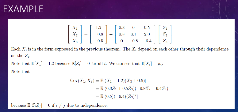
GAUSSIAN VECTORS #

• A random vector $\mathbf{X}=(X_1,\cdots,X_n)$ is said to be Gaussian if $a\cdot\mathbf{X}=a_1X_1+\cdots + a_nX_n$ is Gaussian for any vector $\mathbf{a}=(a_1,\cdots,a_n)$.
  • Recall that if $X_1,\cdots,X_n$ are independent Gaussian variables, then any linear combination $a_1X_1+\cdots + a_nX_n$ is also Gaussian $\Rightarrow\mathbf{X}=X_1,\cdots,X_n$ is Gaussian. The converse is not necessarily true though!
• A random vector $\mathbf{X}=(X_1,\cdots,X_n)$ is Gaussian if and only if it has the form $X_i = \mu_i+\sum_{j = 1}^{n}a_{ij}Z_j$ where $Z_1,\cdots,Z_n$ are independent standard $N(0,1)$ r.v.s.
• If $\mathbf{X}=(X_1,\cdots,X_n)$ is Gaussian, $\mathbf{X}$ and $\mathbf{Y}$ are independent if and only if $\text{Cov}(\mathbf{X},\mathbf{Y}) = 0$. More generally, if $\mathbf{X}$ is Gaussian, then $X_1,\cdots,X_n$ are independent if and only if the covariance matrix is diagonal, that is $\sigma_{ij}=0$ for all $i\neq j$, where $\sigma_{ij}=\text{Cov}(X_i,X_j)$.

GAUSSIAN PROCESSES #

• Let $\mathbf{X}={X_t: t\in T}$ be a stochastic process with state space $\mathbb{R}$ (that is, $X_t\in\mathbb{R}$). Then $\mathbf{X}$ is a Gaussian process if $\mathbf{X}{t_1,\cdots,t_n}=(X{t_1},\cdots,X_{t_n})$ is Gaussian for all choices of $n\geq2$ and $t_1,\cdots,t_n$.
• If $\mathbf{X}$ is a Gaussian process, the distribution of $\mathbf{X}$ is specified for all $n$ and $t_1,\cdots,t_n$ once we specify the mean function $\mu(t)=E[X_t]$ and the covariance function $C(s, t)=\text{Cov}(X_s, X_t)=E[(X_s-\mu(s))(X_t-\mu(t))]=R(s,t)-\mu(s)\cdot\mu(t)$.
  • $\mu(t)$ is arbitrary, but $C(s, t)$ must be symmetric (i.e., $C(s, t)=C(t, s)$, ensure the result is not related to the order of time) and positive-definite.
  • In most applications, $\mu(t)=0$.

DISCRETE TIME STOCHASTIC PROCESSES #

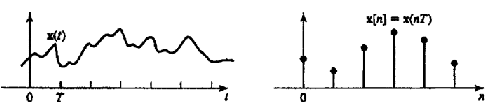
A discrete time stochastic process $\mathbf{X}={X(nT)}$ is a sequence of random variables with mean, autocorrelation and covariance functions:

As before strict-sense stationarity and wide-sense stationarity definitions apply.

• For example, $X(nT)$ is wide-sense stationary if $$ \begin{align*} E\{X(nT)\}&=\mu,\text{ a constant}\\ E\{X((k + n)T)X^*(kT)\}&=R(n)=r_n=r_{-n}^* \end{align*} $$ with $R(n_1,n_2)=R(n_1 - n_2)$ and $n_2 = 0$.

If $X(nT)$ represents a wide-sense stationary input to a discrete-time system $h(nT)$, and $Y(nT)$ the system output, then as before the cross-correlation function satisfies $R_{xy}(n)=R_x(n)*h(-n)$

and the output autocorrelation function is given by

or

Thus wide-sense stationarity from input to output is preserved for discrete-time systems also.

THE DELTA RESPONSE OF A LINEAR DISCRETE SYSTEM #

• The delta response $h[n]$ of a linear system is its response to the delta sequence $\delta[n]$, with system function $H(z)=\sum_{n = -\infty}^{\infty}h[n]z^{-n}$, the $z$-transform of $h[n]$.
• If $x[n]$ is the input to a digital system, the resulting output is the digital convolution of $x[n]$ with $h[n]$: $$ \begin{align*} y[n]&=\sum_{k = -\infty}^{\infty}x[n - k]h[k]=x[n]*h[n]\\ R_{xx}[n_1,n_2]&=\sum_{n = -\infty}^{\infty}x[n_1 - n]x^*[n_2 - n]\\ R_{xy}[n_1,n_2]&=\sum_{n = -\infty}^{\infty}x[n_1 - n]y^*[n_2 - n] \end{align*} $$

Related readings

• Random Walks
• Sequences of Random Variables
• Parameter Estimation
• Two Random Variables
• Random Variables